Tensorflow
[1]:
%matplotlib inline
[2]:
import warnings
warnings.simplefilter('ignore', RuntimeWarning)
[3]:
import matplotlib.pyplot as plt
import pandas as pd
import numpy as np
import seaborn as sns
[4]:
import tensorflow as tf
import tensorflow.keras as keras
Keras
[5]:
Dense = keras.layers.Dense
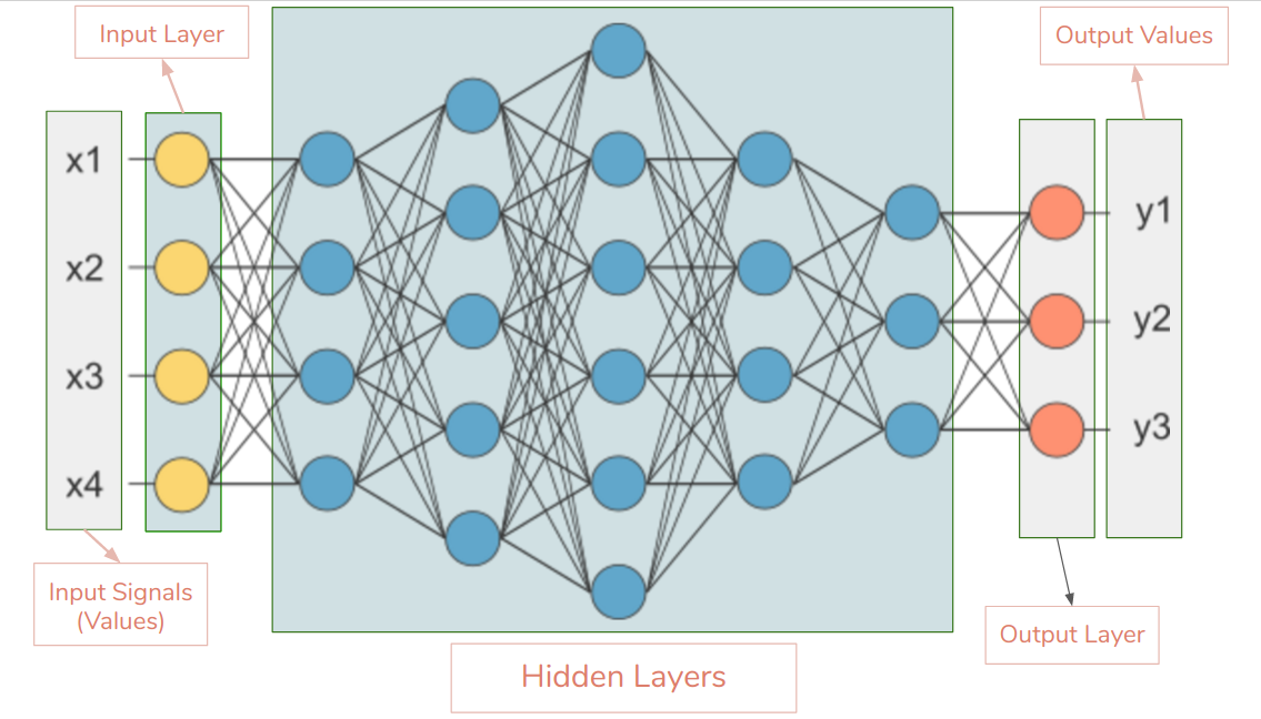
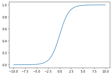
We can consider a DL model as just a black box with a bunch of unnown parameters. For example, when the output is a Dense layer with just one node, the entire network model is just doing some form of regression. If we use a single node with a sigmoid activation function, the model is essentially doing logistic regression.
A single unit with sigmoid activation function
[6]:
X_train = pd.read_csv('data/X_train.csv')
X_test = pd.read_csv('data/X_test.csv')
y_train = pd.read_csv('data/y_train.csv')
y_test = pd.read_csv('data/y_test.csv')
[7]:
X_train.shape
[7]:
(981, 11)
[8]:
model01 = keras.models.Sequential([
    Dense(1,
          activation='sigmoid',
          input_shape=X_train.shape[1:]),
])
[9]:
model01.compile(loss="binary_crossentropy",
                optimizer="sgd",
                metrics=["accuracy"])
[10]:
model01.summary()
Model: "sequential"
_________________________________________________________________
Layer (type)                 Output Shape              Param #
=================================================================
dense (Dense)                (None, 1)                 12
=================================================================
Total params: 12
Trainable params: 12
Non-trainable params: 0
_________________________________________________________________
[11]:
model01.layers
[11]:
[<tensorflow.python.keras.layers.core.Dense at 0x1527d1910>]
[12]:
model01.layers[0].name
[12]:
'dense'
[13]:
model01.layers[0].activation
[13]:
<function tensorflow.python.keras.activations.sigmoid(x)>
[14]:
hist = model01.fit(X_train,
                   y_train,
                   epochs=20,
                   verbose=0,
                   validation_split=0.2)
[15]:
import pandas as pd
[16]:
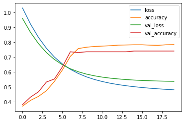
df = pd.DataFrame(hist.history)
[17]:
df.head()
[17]:
| loss | accuracy | val_loss | val_accuracy | |
|---|---|---|---|---|
| 0 | 1.029838 | 0.371173 | 0.959598 | 0.380711 |
| 1 | 0.922509 | 0.409439 | 0.866757 | 0.431472 |
| 2 | 0.833006 | 0.436224 | 0.791162 | 0.467005 |
| 3 | 0.759757 | 0.474490 | 0.730747 | 0.532995 |
| 4 | 0.700539 | 0.536990 | 0.684353 | 0.553299 |
[18]:
df.plot()
pass
[19]:
model01.evaluate(X_test, y_test)
11/11 [==============================] - 0s 591us/step - loss: 0.4566 - accuracy: 0.8293
[19]:
[0.4565536081790924, 0.8292682766914368]
[20]:
k = 5
np.c_[model01.predict(X_test.iloc[:k, :]), y_test[:k]]
[20]:
array([[0.71404094, 0.        ],
       [0.17881006, 0.        ],
       [0.56976336, 1.        ],
       [0.33437088, 1.        ],
       [0.87005341, 1.        ]])
Saving and loading model weights
[21]:
model01.save('titanic.h5')
[22]:
model011A = keras.models.load_model('titanic.h5')
[23]:
model011A.summary()
Model: "sequential"
_________________________________________________________________
Layer (type)                 Output Shape              Param #
=================================================================
dense (Dense)                (None, 1)                 12
=================================================================
Total params: 12
Trainable params: 12
Non-trainable params: 0
_________________________________________________________________
Logistic regression replicates results
[24]:
import h5py
[25]:
fh = h5py.File('titanic.h5', 'r')
[26]:
fh.keys()
[26]:
<KeysViewHDF5 ['model_weights', 'optimizer_weights']>
[27]:
fh['model_weights'].keys()
[27]:
<KeysViewHDF5 ['dense']>
[28]:
fh['model_weights'].get('dense').get('dense').keys()
[28]:
<KeysViewHDF5 ['bias:0', 'kernel:0']>
[29]:
bias = fh['model_weights'].get('dense').get('dense').get('bias:0')
bias
[29]:
<HDF5 dataset "bias:0": shape (1,), type "<f4">
[30]:
wts = fh['model_weights'].get('dense').get('dense').get('kernel:0')
wts
[30]:
<HDF5 dataset "kernel:0": shape (11, 1), type "<f4">
[31]:
bias[:]
[31]:
array([-0.4318819], dtype=float32)
[32]:
wts[:]
[32]:
array([[-0.26382327],
       [ 0.11888377],
       [ 1.0947229 ],
       [-0.20582937],
       [-0.35638043],
       [ 0.02472745],
       [ 0.10281957],
       [ 0.03278307],
       [-0.25210753],
       [-0.26847404],
       [ 0.09856348]], dtype=float32)
[33]:
logodds = bias[:] + X_test.iloc[:5, :] @ wts[:]
odds = np.exp(logodds)
p_lr = odds/(1 + odds)
[34]:
p_nn = model01.predict(X_test.iloc[:5])
[35]:
pd.DataFrame(np.c_[p_lr, p_nn], columns=['lr', 'nn'])
[35]:
| lr | nn | |
|---|---|---|
| 0 | 0.714041 | 0.714041 |
| 1 | 0.178810 | 0.178810 |
| 2 | 0.569763 | 0.569763 |
| 3 | 0.334371 | 0.334371 |
| 4 | 0.870053 | 0.870053 |
[36]:
fh.close()
Building blocks
A keras model is composed of layers. Each layer has its own activation function. Each layer also has its own biases and weights. To set initial random weights, there are several possible strategies known as initializers. To fit the model, you need to specify a loss function. During training, the optimizer finds biases and weights that minimize the loss function. Model performance is evaluated using metrics.
Commonly used versions of these classes or functions come built-in with keras.
Layers
[37]:
[x for x in dir(keras.layers) if
 x[0].isupper() and
 not x.startswith('_')]
[37]:
['AbstractRNNCell',
 'Activation',
 'ActivityRegularization',
 'Add',
 'AdditiveAttention',
 'AlphaDropout',
 'Attention',
 'Average',
 'AveragePooling1D',
 'AveragePooling2D',
 'AveragePooling3D',
 'AvgPool1D',
 'AvgPool2D',
 'AvgPool3D',
 'BatchNormalization',
 'Bidirectional',
 'Concatenate',
 'Conv1D',
 'Conv1DTranspose',
 'Conv2D',
 'Conv2DTranspose',
 'Conv3D',
 'Conv3DTranspose',
 'ConvLSTM2D',
 'Convolution1D',
 'Convolution1DTranspose',
 'Convolution2D',
 'Convolution2DTranspose',
 'Convolution3D',
 'Convolution3DTranspose',
 'Cropping1D',
 'Cropping2D',
 'Cropping3D',
 'Dense',
 'DenseFeatures',
 'DepthwiseConv2D',
 'Dot',
 'Dropout',
 'ELU',
 'Embedding',
 'Flatten',
 'GRU',
 'GRUCell',
 'GaussianDropout',
 'GaussianNoise',
 'GlobalAveragePooling1D',
 'GlobalAveragePooling2D',
 'GlobalAveragePooling3D',
 'GlobalAvgPool1D',
 'GlobalAvgPool2D',
 'GlobalAvgPool3D',
 'GlobalMaxPool1D',
 'GlobalMaxPool2D',
 'GlobalMaxPool3D',
 'GlobalMaxPooling1D',
 'GlobalMaxPooling2D',
 'GlobalMaxPooling3D',
 'Input',
 'InputLayer',
 'InputSpec',
 'LSTM',
 'LSTMCell',
 'Lambda',
 'Layer',
 'LayerNormalization',
 'LeakyReLU',
 'LocallyConnected1D',
 'LocallyConnected2D',
 'Masking',
 'MaxPool1D',
 'MaxPool2D',
 'MaxPool3D',
 'MaxPooling1D',
 'MaxPooling2D',
 'MaxPooling3D',
 'Maximum',
 'Minimum',
 'Multiply',
 'PReLU',
 'Permute',
 'RNN',
 'ReLU',
 'RepeatVector',
 'Reshape',
 'SeparableConv1D',
 'SeparableConv2D',
 'SeparableConvolution1D',
 'SeparableConvolution2D',
 'SimpleRNN',
 'SimpleRNNCell',
 'Softmax',
 'SpatialDropout1D',
 'SpatialDropout2D',
 'SpatialDropout3D',
 'StackedRNNCells',
 'Subtract',
 'ThresholdedReLU',
 'TimeDistributed',
 'UpSampling1D',
 'UpSampling2D',
 'UpSampling3D',
 'Wrapper',
 'ZeroPadding1D',
 'ZeroPadding2D',
 'ZeroPadding3D']
Activations
[38]:
[x for x in dir(keras.activations) if
 x[0].islower() and
 not x.startswith('_')]
[38]:
['deserialize',
 'elu',
 'exponential',
 'get',
 'hard_sigmoid',
 'linear',
 'relu',
 'selu',
 'serialize',
 'sigmoid',
 'softmax',
 'softplus',
 'softsign',
 'swish',
 'tanh']
Initializers
[41]:
[x for x in dir(keras.initializers) if
 x[0].isupper() and
 not x.startswith('_')]
[41]:
['Constant',
 'GlorotNormal',
 'GlorotUniform',
 'HeNormal',
 'HeUniform',
 'Identity',
 'Initializer',
 'LecunNormal',
 'LecunUniform',
 'Ones',
 'Orthogonal',
 'RandomNormal',
 'RandomUniform',
 'TruncatedNormal',
 'VarianceScaling',
 'Zeros']
Example
[42]:
init = keras.initializers.LecunNormal(seed=0)
init(shape=(2,3)).numpy()
[42]:
array([[-1.3641988 , -0.38696545, -0.532354  ],
       [ 0.06994588, -0.21366763,  0.07270983]], dtype=float32)
Losses
[43]:
[x for x in dir(keras.losses) if
 x[0].isupper() and
 not x.startswith('_')]
[43]:
['BinaryCrossentropy',
 'CategoricalCrossentropy',
 'CategoricalHinge',
 'CosineSimilarity',
 'Hinge',
 'Huber',
 'KLD',
 'KLDivergence',
 'LogCosh',
 'Loss',
 'MAE',
 'MAPE',
 'MSE',
 'MSLE',
 'MeanAbsoluteError',
 'MeanAbsolutePercentageError',
 'MeanSquaredError',
 'MeanSquaredLogarithmicError',
 'Poisson',
 'Reduction',
 'SparseCategoricalCrossentropy',
 'SquaredHinge']
Example
[44]:
loss = keras.losses.BinaryCrossentropy()
[45]:
y_true = [1,0,0,1]
y_pred = [0.9, 0.2, 0.3, 0.8]
loss(y_true, y_pred).numpy()
[45]:
0.2270805
Metrics
[46]:
[x for x in dir(keras.metrics) if
 x[0].isupper() and
 not x.startswith('_')]
[46]:
['AUC',
 'Accuracy',
 'BinaryAccuracy',
 'BinaryCrossentropy',
 'CategoricalAccuracy',
 'CategoricalCrossentropy',
 'CategoricalHinge',
 'CosineSimilarity',
 'FalseNegatives',
 'FalsePositives',
 'Hinge',
 'KLD',
 'KLDivergence',
 'LogCoshError',
 'MAE',
 'MAPE',
 'MSE',
 'MSLE',
 'Mean',
 'MeanAbsoluteError',
 'MeanAbsolutePercentageError',
 'MeanIoU',
 'MeanRelativeError',
 'MeanSquaredError',
 'MeanSquaredLogarithmicError',
 'MeanTensor',
 'Metric',
 'Poisson',
 'Precision',
 'PrecisionAtRecall',
 'Recall',
 'RecallAtPrecision',
 'RootMeanSquaredError',
 'SensitivityAtSpecificity',
 'SparseCategoricalAccuracy',
 'SparseCategoricalCrossentropy',
 'SparseTopKCategoricalAccuracy',
 'SpecificityAtSensitivity',
 'SquaredHinge',
 'Sum',
 'TopKCategoricalAccuracy',
 'TrueNegatives',
 'TruePositives']
Example
[47]:
metric = keras.metrics.Accuracy()
[48]:
metric.reset_states()
[49]:
metric.update_state(
    [[1], [2], [3]],
    [[1], [1], [3]]
)
[49]:
<tf.Variable 'UnreadVariable' shape=() dtype=float32, numpy=3.0>
[50]:
metric.result().numpy()
[50]:
0.6666667
Optimizers
[51]:
[x for x in dir(keras.optimizers) if
 x[0].isupper() and
 not x.startswith('_')]
[51]:
['Adadelta',
 'Adagrad',
 'Adam',
 'Adamax',
 'Ftrl',
 'Nadam',
 'Optimizer',
 'RMSprop',
 'SGD']
Example
[52]:
opt = keras.optimizers.Adam(learning_rate=0.1)
[53]:
v = tf.Variable(10.0)
loss = lambda: v**2/2.0
n_steps = opt.minimize(loss, [v]).numpy()
[54]:
v.numpy()
[54]:
9.9
[55]:
n_steps = opt.minimize(loss, [v]).numpy()
[56]:
v.numpy()
[56]:
9.800028
[57]:
n_steps
[57]:
2
Tensorflow Datasets Project
Makes it simple to download standard datasets for deep learning.
[58]:
! python3 -m pip install --quiet tensorflow-datasets
[59]:
import tensorflow_datasets as tfds
[60]:
ds, info = tfds.load(name='fashion_mnist',
                     as_supervised=True,
                     with_info=True)
[61]:
ds
[61]:
{'test': <PrefetchDataset shapes: ((28, 28, 1), ()), types: (tf.uint8, tf.int64)>,
 'train': <PrefetchDataset shapes: ((28, 28, 1), ()), types: (tf.uint8, tf.int64)>}
[62]:
info
[62]:
tfds.core.DatasetInfo(
name='fashion_mnist',
version=3.0.1,
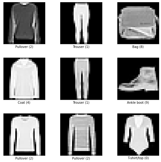
description='Fashion-MNIST is a dataset of Zalando's article images consisting of a training set of 60,000 examples and a test set of 10,000 examples. Each example is a 28x28 grayscale image, associated with a label from 10 classes.',
homepage='https://github.com/zalandoresearch/fashion-mnist',
features=FeaturesDict({
'image': Image(shape=(28, 28, 1), dtype=tf.uint8),
'label': ClassLabel(shape=(), dtype=tf.int64, num_classes=10),
}),
total_num_examples=70000,
splits={
'test': 10000,
'train': 60000,
},
supervised_keys=('image', 'label'),
citation="""@article{DBLP:journals/corr/abs-1708-07747,
author = {Han Xiao and
Kashif Rasul and
Roland Vollgraf},
title = {Fashion-MNIST: a Novel Image Dataset for Benchmarking Machine Learning
Algorithms},
journal = {CoRR},
volume = {abs/1708.07747},
year = {2017},
url = {http://arxiv.org/abs/1708.07747},
archivePrefix = {arXiv},
eprint = {1708.07747},
timestamp = {Mon, 13 Aug 2018 16:47:27 +0200},
biburl = {https://dblp.org/rec/bib/journals/corr/abs-1708-07747},
bibsource = {dblp computer science bibliography, https://dblp.org}
}""",
redistribution_info=,
)
[63]:
X_train, X_test = ds['train'], ds['test']
[64]:
#### Displaying the dataset
[65]:
tfds.as_dataframe(X_train.take(5), info)
[65]:
| image | label | |
|---|---|---|
| 0 |  |
2 (Pullover) |
| 1 |  |
1 (Trouser) |
| 2 |  |
8 (Bag) |
| 3 |  |
4 (Coat) |
| 4 |  |
1 (Trouser) |
[66]:
tfds.show_examples(X_train, info);
Feed into deep learning pipeline
The data is ready to be fed to a keras model.
Coming in next lecture.