Random Numbers
Pseudorandom number generators (PRNG)
While psuedorandom numbers are generated by a deterministic algorithm, we can mostly treat them as if they were true random numbers and we will drop the “pseudo” prefix. Fundamentally, the algorithm generates random integers which are then normalized to give a floating point number from the standard uniform distribution. Random numbers from other distributions are in turn generated using these uniform random deviates, either via general (inverse transform, accept/reject, mixture representations) or specialized ad-hoc (e.g. Box-Muller) methods.
Generating standard uniform random numbers
Linear congruential generators (LCG)
\(z_{i+1} = (az_i + c) \mod m\)
Hull-Dobell Theorem: The LCG will have a full period for all seeds if and only if
- \(c\) and \(m\) are relatively prime,
- \(a - 1\) is divisible by all prime factors of \(m\)
- \(a - 1\) is a multiple of 4 if \(m\) is a multiple of 4.
The number \(z_0\) is called the seed, and setting it allows us to have a reproducible sequence of “random” numbers. The LCG is typically coded to return \(z/m\), a floating point number in (0, 1). This can be scaled to any other range \((a, b)\).
Note that most PRNGs now use the Mersenne twister, but the LCG is presented because the LCG code much easier to understand and all we hope for is some appreciation for how apparently random sequences can be generated from a deterministic iterative scheme.
In [2]:
def rng(m=2**32, a=1103515245, c=12345):
    rng.current = (a*rng.current + c) % m
    return rng.current/m

# setting the seed
rng.current = 1
In [3]:
[rng() for i in range(10)]
Out[3]:
[0.25693503906950355,
 0.5878706516232342,
 0.15432575810700655,
 0.767266943352297,
 0.9738139626570046,
 0.5858681506942958,
 0.8511155843734741,
 0.6132153405342251,
 0.7473867232911289,
 0.06236015981994569]
From standard uniform to other distributions
Inverse transform method
Once we have standard uniform numbers, we can often generate random numbers from other distribution using the inverse transform method. Recall that if \(X\) is a continuous random variable with CDF \(F_X\), then \(Y = F_X(X)\) has the standard uniform distribution. Inverting this suggests that if \(Y\) comes from a standard uniform distribution, then \(F_X^{-1}(Y)\) has the same distribution as \(X\). The inverse transform method is used below to generate random numbers from the exponential distribution.
In [5]:
def expon_pdf(x, lmabd=1):
    """PDF of exponential distribution."""
    return lmabd*np.exp(-lmabd*x)
In [6]:
def expon_cdf(x, lambd=1):
    """CDF of exponetial distribution."""
    return 1 - np.exp(-lambd*x)
In [7]:
def expon_icdf(p, lambd=1):
    """Inverse CDF of exponential distribution - i.e. quantile function."""
    return -np.log(1-p)/lambd
In [9]:
import scipy.stats as stats

dist = stats.expon()
x = np.linspace(0,4,100)
y = np.linspace(0,1,100)

with plt.xkcd():
    plt.figure(figsize=(12,4))
    plt.subplot(121)
    plt.plot(x, expon_cdf(x))
    plt.axis([0, 4, 0, 1])
    for q in [0.5, 0.8]:
        plt.arrow(0, q, expon_icdf(q)-0.1, 0, head_width=0.05, head_length=0.1, fc='b', ec='b')
        plt.arrow(expon_icdf(q), q, 0, -q+0.1, head_width=0.1, head_length=0.05, fc='b', ec='b')
    plt.ylabel('1: Generate a (0,1) uniform PRNG')
    plt.xlabel('2: Find the inverse CDF')
    plt.title('Inverse transform method');

    plt.subplot(122)
    u = np.random.random(10000)
    v = expon_icdf(u)
    plt.hist(v, histtype='step', bins=100, normed=True, linewidth=2)
    plt.plot(x, expon_pdf(x), linewidth=2)
    plt.axis([0,4,0,1])
    plt.title('Histogram of exponential PRNGs');

Creating a random number generator for arbitrary distributions
Suppose we have some random samples with an unknown distribution. We can still use the inverse transform method to create a random number generator from a random sample, by estimating the inverse CDF function using interpolation.
In [11]:
from scipy.interpolate import interp1d
from statsmodels.distributions.empirical_distribution import ECDF

# Make up some random data
x = np.concatenate([np.random.normal(0, 1, 10000),
                    np.random.normal(4, 1, 10000)])

ecdf = ECDF(x)
inv_cdf = interp1d(ecdf.y, ecdf.x, bounds_error=False, assume_sorted=True)
r = np.random.uniform(0, 1, 1000)
ys = inv_cdf(r)

plt.hist(x, 25, histtype='step', color='red', normed=True, linewidth=1)
plt.hist(ys, 25, histtype='step', color='blue', normed=True, linewidth=1);

Rejection sampling (Accept-reject method)
In [13]:
# Suppose we want to sample from the (truncated) T distribution witb 10 degrees of freedom
# We use the uniform as a proposal distibution (highly inefficient)

x = np.linspace(-4, 4)

df = 10
dist = stats.cauchy()
upper = dist.pdf(0)

with plt.xkcd():
    plt.figure(figsize=(12,4))
    plt.subplot(121)
    plt.plot(x, dist.pdf(x))
    plt.axhline(upper, color='grey')
    px = 1.0
    plt.arrow(px,0,0,dist.pdf(1.0)-0.01, linewidth=1,
              head_width=0.2, head_length=0.01, fc='g', ec='g')
    plt.arrow(px,upper,0,-(upper-dist.pdf(px)-0.01), linewidth=1,
              head_width=0.3, head_length=0.01, fc='r', ec='r')
    plt.text(px+.25, 0.2, 'Reject', fontsize=16)
    plt.text(px+.25, 0.01, 'Accept', fontsize=16)
    plt.axis([-4,4,0,0.4])
    plt.title('Rejection sampling concepts', fontsize=20)

    plt.subplot(122)
    n = 100000
    # generate from sampling distribution
    u = np.random.uniform(-4, 4, n)
    # accept-reject criterion for each point in sampling distribution
    r = np.random.uniform(0, upper, n)
    # accepted points will come from target (Cauchy) distribution
    v = u[r < dist.pdf(u)]

    plt.plot(x, dist.pdf(x), linewidth=2)

    # Plot scaled histogram
    factor = dist.cdf(4) - dist.cdf(-4)
    hist, bin_edges = np.histogram(v, bins=100, normed=True)
    bin_centers = (bin_edges[:-1] + bin_edges[1:]) / 2.
    plt.step(bin_centers, factor*hist, linewidth=2)

    plt.axis([-4,4,0,0.4])
    plt.title('Histogram of accepted samples', fontsize=20);

Mixture representations
Sometimes, the target distribution from which we need to generate random numbers can be expressed as a mixture of “simpler” distributions that we already know how to sample from
For example, if \(y\) is drawn from the \(\chi_\nu^2\) distribution, then \(\mathcal{N}(0, \nu/y)\) is a sample from the Student’s T distribution with \(\nu\) degrees of freedom.
In [23]:
n = 10000
df = 2
dist = stats.t(df=df)
y = stats.chi2(df=df).rvs(n)
r = stats.norm(0, df/y).rvs(n)

with plt.xkcd():
    plt.plot(x, dist.pdf(x), linewidth=2)

    # Plot scaled histogram
    factor = dist.cdf(4) - dist.cdf(-4)
    hist, bin_edges = np.histogram(v, bins=100, normed=True)
    bin_centers = (bin_edges[:-1] + bin_edges[1:]) / 2.
    plt.step(bin_centers, factor*hist, linewidth=2)

    plt.axis([-4,4,0,0.4])
    plt.title('Histogram of accepted samples', fontsize=20);

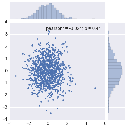
Ad-hoc methods - e.g. Box-Muller for generating normally distributed random numbers
The Box-Muller transform starts with 2 random uniform numbers \(u\) and \(v\) - Generate an exponentially distributed variable \(r^2\) from \(u\) using the inverse transform method - This means that \(r\) is an exponentially distributed variable on \((0, \infty)\) - Generate a variable \(\theta\) uniformly distributed on \((0, 2\pi)\) from \(v\) by scaling - In polar coordinates, the vector \((r, \theta)\) has an independent bivariate normal distribution - Hence the projection onto the \(x\) and \(y\) axes give independent univariate normal random numbers
Note:
- Normal random numbers can also be generated using the general inverse transform method (e.g. by approximating the inverse CDF with a polynomial) or the rejection method (e.g. using the exponential distribution as the sampling distribution).
- There is also a variant of Box-Muller that does not require the use of (expensive) trigonometric calculations.
In [24]:
n = 1000
u1 = np.random.random(n)
u2 = np.random.random(n)
r_squared = -2*np.log(u1)
r = np.sqrt(r_squared)
theta = 2*np.pi*u2
x = r*np.cos(theta)
y = r*np.sin(theta)
In [25]:
sns.jointplot(x, y, kind='scatter')
pass
Using the numpy.random and scipy.stats PRNGs
From this part onwards, we will assume that there is a library of PRNGs
that we can use - either from numpy.random or scipy.stats which are
both based on the Mersenne Twister, a high-quality PRNG for random
integers. The numpy versions simply generate random deviates while
the scipy versions will also provide useful functions related to the
distribution, e.g. PDF, CDF and quantiles.
In [35]:
import numpy.random as rng

# Histogram of beta distribution
rs = rng.beta(a=0.5, b=0.5, size=1000)
plt.hist(rs, bins=20, histtype='step', normed=True, linewidth=1)

# PDF for the beta distribution
xs = np.linspace(0, 1, 100)
plt.plot(xs, stats.beta.pdf(xs, a=0.5, b=0.5), color='red')
pass

In [27]:
%load_ext rpy2.ipython
In [30]:
%%R

n <- 5
xs <- c(0.1, 0.5, 0.9)
print(dbeta(xs, 0.5, 0.5))
print(pbeta(xs, 0.5, 0.5))
print(qbeta(xs, 0.5, 0.5))
print(rbeta(n, 0.5, 0.5))
[1] 1.0610330 0.6366198 1.0610330
[1] 0.2048328 0.5000000 0.7951672
[1] 0.02447174 0.50000000 0.97552826
[1] 0.9685769 0.6340875 0.9386236 0.3633199 0.6934238
In [33]:
# Using scipy

n = 5
xs = [0.1, 0.5, 0.9]
rv = stats.beta(a=0.5, b=0.5)

print(rv.pdf(xs)) # equivalent of dbeta
print(rv.cdf(xs)) # equivalent of pbeta
print(rv.ppf(xs)) # equvialent of qbeta
print(rv.rvs(n)) # equivalent of rbeta
[ 1.06103295  0.63661977  1.06103295]
[ 0.20483276  0.5         0.79516724]
[ 0.02447174  0.5         0.97552826]
[ 0.09332562  0.21171851  0.42106969  0.76274382  0.890998  ]