Using PyMC3
PyMC3 is a Python package for doing MCMC using a variety of samplers, including Metropolis, Slice and Hamiltonian Monte Carlo. See Probabilistic Programming in Python using PyMC for a description. The GitHub site also has many examples and links for further exploration.
In [1]:
! pip install --quiet pymc3
! pip install --quiet daft
! pip install --quiet seaborn
In [2]:
! conda install --yes --quiet mkl-service
Fetching package metadata .........
Solving package specifications: ..........

# All requested packages already installed.
# packages in environment at /opt/conda:
#
mkl-service               1.1.2                    py35_3
Other resources
Some examples are adapted from:
In [3]:
%matplotlib inline
In [4]:
import numpy as np
import numpy.random as rng
import matplotlib.pyplot as plt
import seaborn as sns
import pandas as pd
import pymc3 as pm
import scipy.stats as stats
from sklearn.preprocessing import StandardScaler
import daft
In [5]:
import theano
theano.config.warn.round=False
Example: Estimating coin bias
We start with the simplest model - that of determining the bias of a coin from observed outcomes.
Setting up the model
In [6]:
n = 100
heads = 61
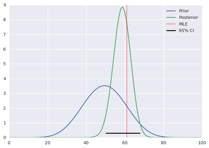
Analytical solution
In [7]:
a, b = 10, 10
prior = stats.beta(a, b)
post = stats.beta(heads+a, n-heads+b)
ci = post.interval(0.95)

xs = np.linspace(0, 1, 100)
plt.plot(prior.pdf(xs), label='Prior')
plt.plot(post.pdf(xs), label='Posterior')
plt.axvline(100*heads/n, c='red', alpha=0.4, label='MLE')
plt.xlim([0, 100])
plt.axhline(0.3, ci[0], ci[1], c='black', linewidth=2, label='95% CI');
plt.legend()
pass
Graphical model
In [8]:
pgm = daft.PGM(shape=[2.5, 3.0], origin=[0, -0.5])

pgm.add_node(daft.Node("alpha", r"$\alpha$", 0.5, 2, fixed=True))
pgm.add_node(daft.Node("beta", r"$\beta$", 1.5, 2, fixed=True))
pgm.add_node(daft.Node("p", r"$p$", 1, 1))
pgm.add_node(daft.Node("n", r"$n$", 2, 0, fixed=True))
pgm.add_node(daft.Node("y", r"$y$", 1, 0, observed=True))

pgm.add_edge("alpha", "p")
pgm.add_edge("beta", "p")
pgm.add_edge("n", "y")
pgm.add_edge("p", "y")

pgm.render()
pass

Introduction to PyMC3
In [9]:
niter = 2000
with pm.Model() as coin_context:
    p = pm.Beta('p', alpha=2, beta=2)
    y = pm.Binomial('y', n=n, p=p, observed=heads)
    trace = pm.sample(niter)
Auto-assigning NUTS sampler...
Initializing NUTS using advi...
Average ELBO = -4.2744: 100%|██████████| 200000/200000 [00:15<00:00, 12698.15it/s]
Finished [100%]: Average ELBO = -4.2693
100%|██████████| 2000/2000 [00:01<00:00, 1753.85it/s]
Specifying start, sampler (step) and multiple chains
In [10]:
with coin_context:
    start = pm.find_MAP()
    step = pm.Metropolis()
    trace = pm.sample(niter, step=step, start=start, njobs=4, random_seed=123)
Optimization terminated successfully.
         Current function value: 3.582379
         Iterations: 3
         Function evaluations: 5
         Gradient evaluations: 5
100%|██████████| 2000/2000 [00:00<00:00, 5656.17it/s]
Summary of results
Getting values from the trace
In [13]:
p = trace.get_values('p', burn=niter//2, combine=True, chains=[0,2])
p.shape
Out[13]:
(2000,)

Calculate effective sample size
where \(m\) is the number of chains, \(n\) the number of steps per chain, \(T\) the time when the autocorrelation first becomes negative, and \(\hat{\rho}_t\) the autocorrelation at lag \(t\).
In [15]:
pm.effective_n(t)
Out[15]:
{'p': 767.0, 'p_logodds_': 765.0}
Evaluate convergence
where \(W\) is the within-chain variance and \(\hat{V}\) is the posterior variance estimate for the pooled traces. Values greater than one indicate that one or more chains have not yet converged.
Discrad burn-in steps for each chain. The idea is to see if the starting values of each chain come from the same distribution as the stationary state.
- \(W\) is the number of chains \(m \times\) the variacne of each individual chain
- \(B\) is the number of steps \(n \times\) the variance of the chain means
- \(\hat{V}\) is the weigthed average \((1 - \frac{1}{n})W + \frac{1}{n}B\)
The idea is that \(\hat{V}\) is an unbiased estimator of \(W\) if the starting values of each chain come from the same distribution as the stationary state. Hence if \(\hat{R}\) differs significantly from 1, there is probsbly no convergence and we need more iterations. This is done for each parameter \(\theta\).
In [16]:
pm.gelman_rubin(t)
Out[16]:
{'p': 0.99949987493746084, 'p_logodds_': 0.99949987493746095}
Compares mean of initial with later segments of a trace for a parameter. Should have absolute value less than 1 at convergence.
In [17]:
plt.plot(pm.geweke(t['p'])[:,1], 'o')
plt.axhline(1, c='red')
plt.axhline(-1, c='red')
plt.gca().margins(0.05)
pass

In [18]:
pm.summary(t, varnames=['p'])
p:

  Mean             SD               MC Error         95% HPD interval
  -------------------------------------------------------------------

  0.615            0.050            0.002            [0.517, 0.698]

  Posterior quantiles:
  2.5            25             50             75             97.5
  |--------------|==============|==============|--------------|

  0.517          0.581          0.616          0.654          0.698
In [19]:
pm.traceplot(t, varnames=['p'])
pass

In [20]:
with coin_context:
    ppc = pm.sample_ppc(t, samples=100)
ppc['y'].ravel()
100%|██████████| 100/100 [00:00<00:00, 337.12it/s]
Out[20]:
array([67, 70, 53, 66, 41, 56, 70, 60, 66, 46, 48, 63, 64, 58, 65, 55, 63,
       66, 67, 58, 70, 73, 69, 55, 51, 70, 58, 68, 59, 50, 60, 67, 59, 58,
       70, 56, 62, 63, 68, 65, 60, 64, 58, 44, 68, 75, 60, 55, 64, 66, 71,
       59, 62, 53, 62, 67, 65, 59, 56, 59, 62, 67, 61, 58, 79, 68, 54, 62,
       71, 60, 66, 57, 67, 70, 47, 58, 69, 68, 62, 67, 49, 61, 66, 40, 57,
       65, 53, 40, 67, 65, 55, 53, 70, 61, 57, 51, 66, 68, 68, 73])
Saving traces
In [21]:
from pymc3.backends import Text

niter = 2000
with pm.Model() as text_save_demo:
    p = pm.Beta('p', alpha=2, beta=2)
    y = pm.Binomial('y', n=n, p=p, observed=heads)
    db = Text('trace')
    trace = pm.sample(niter, trace=db)
Auto-assigning NUTS sampler...
Initializing NUTS using advi...
Average ELBO = -4.2758: 100%|██████████| 200000/200000 [00:16<00:00, 12263.44it/s]
Finished [100%]: Average ELBO = -4.2726
100%|██████████| 2000/2000 [00:01<00:00, 1655.80it/s]
In [22]:
with text_save_demo:
    trace = pm.backends.text.load('trace')
    pm.traceplot(trace, varnames=['p'])

In [23]:
trace.varnames
Out[23]:
['p_logodds_', 'p']
If you are fitting a large complex model that may not fit in memory, you can use the SQLite3 backend to save the trace incremnetally to disk.
In [24]:
from pymc3.backends import SQLite

niter = 2000
with pm.Model() as sqlie3_save_demo:
    p = pm.Beta('p', alpha=2, beta=2)
    y = pm.Binomial('y', n=n, p=p, observed=heads)
    db = SQLite('trace.db')
    trace = pm.sample(niter, trace=db)
Auto-assigning NUTS sampler...
Initializing NUTS using advi...
Average ELBO = -4.2776: 100%|██████████| 200000/200000 [00:17<00:00, 11746.28it/s]
Finished [100%]: Average ELBO = -4.2749
100%|██████████| 2000/2000 [00:01<00:00, 1496.41it/s]
In [25]:
with sqlie3_save_demo:
    trace = pm.backends.sqlite.load('trace.db')
    pm.traceplot(trace, varnames=['p'])

Sampling from prior
Just omit the observed= argument.
In [26]:
with pm.Model() as prior_context:
    sigma = pm.Gamma('sigma', alpha=2.0, beta=1.0)
    mu = pm.Normal('mu', mu=0, sd=sigma)
    trace = pm.sample(niter, step=pm.Metropolis())
100%|██████████| 2000/2000 [00:00<00:00, 4522.74it/s]
In [27]:
pm.traceplot(trace, varnames=['mu', 'sigma'])
pass

Univariate normal distribution
In [28]:
xs = rng.normal(loc=5, scale=2, size=100)
In [29]:
sns.distplot(xs, rug=True)
pass
/opt/conda/lib/python3.5/site-packages/statsmodels/nonparametric/kdetools.py:20: VisibleDeprecationWarning: using a non-integer number instead of an integer will result in an error in the future
  y = X[:m/2+1] + np.r_[0,X[m/2+1:],0]*1j

Sampling from posterior
In [30]:
niter = 2000
with pm.Model() as normal_context:
    mu = pm.Normal('mu', mu=0, sd=100)
    sd = pm.HalfCauchy('sd', beta=2)
    y = pm.Normal('y', mu=mu, sd=sd, observed=xs)
    trace = pm.sample(niter)
Auto-assigning NUTS sampler...
Initializing NUTS using advi...
Average ELBO = -223.18: 100%|██████████| 200000/200000 [00:19<00:00, 10185.34it/s]
Finished [100%]: Average ELBO = -223.18
100%|██████████| 2000/2000 [00:02<00:00, 847.15it/s]
In [31]:
hpd = pm.stats.hpd(trace, alpha=0.05)
hpd
Out[31]:
{'mu': array([ 4.87008876,  5.68313862]),
 'sd': array([ 1.80810522,  2.38210096]),
 'sd_log_': array([ 0.59227946,  0.86798286])}
In [32]:
ax = pm.traceplot(trace, varnames=['mu', 'sd'],)

ymin, ymax = ax[0,0].get_ylim()
y = ymin + 0.05*(ymax-ymin)
ax[0, 0].plot(hpd['mu'], [y,y], c='red')

ymin, ymax = ax[1,0].get_ylim()
y = ymin + 0.05*(ymax-ymin)
ax[1, 0].plot(hpd['sd'], [y,y], c='red')
pass

Evaluating goodness-of-fit
DIC, WAIC and BPIC are approximations to the out-of-sample error and can be used for model comparison. Likelihood is dependent on model complexity and should not be used for model comparisons.
In [33]:
post_mean = pm.df_summary(trace, varnames=trace.varnames)['mean'].to_dict()
post_mean
Out[33]:
{'mu': 5.2774425669706622,
 'sd': 2.083811018098618,
 'sd_log_': 0.73163253719625909}
In [34]:
normal_context.logp(post_mean)
Out[34]:
array(-220.7824869198777)
In [35]:
with normal_context:
    print(pm.stats.dic(trace))
445.508693887
In [36]:
with normal_context:
    print(pm.stats.waic(trace))
(432.18295932008124, 14.386599474961665)
In [37]:
with normal_context:
    print(pm.stats.bpic(trace))
447.480553911
Linear regression
We will show how to estimate regression parameters using a simple linear model
We can restate the linear model
as sampling from a probability distribution
Now we can use pymc to estimate the parameters \(a\), \(b\)
and \(\sigma\). We will assume the following priors
In [38]:
import daft

# Instantiate the PGM.
pgm = daft.PGM(shape=[4.0, 3.0], origin=[-0.3, -0.7])

# Hierarchical parameters.
pgm.add_node(daft.Node("alpha", r"$\alpha$", 0.5, 2))
pgm.add_node(daft.Node("beta", r"$\beta$", 1.5, 2))
pgm.add_node(daft.Node("sigma", r"$\sigma$", 0, 0))

# Deterministic variable.
pgm.add_node(daft.Node("mu", r"$\mu_n$", 1, 1))

# Data.
pgm.add_node(daft.Node("x", r"$x_n$", 2, 1, observed=True))
pgm.add_node(daft.Node("y", r"$y_n$", 1, 0, observed=True))

# Add in the edges.
pgm.add_edge("alpha", "mu")
pgm.add_edge("beta", "mu")
pgm.add_edge("x", "mu")
pgm.add_edge("mu", "y")
pgm.add_edge("sigma", "y")

# And a plate.
pgm.add_plate(daft.Plate([0.5, -0.5, 2, 2], label=r"$n = 1, \cdots, N$",
    shift=-0.1))

# Render and save.
pgm.render()
pgm.figure.savefig("lm.pdf")

In [39]:
# observed data
np.random.seed(123)
n = 11
_a = 6
_b = 2
x = np.linspace(0, 1, n)
y = _a*x + _b + np.random.randn(n)
In [40]:
niter = 10000
with pm.Model() as linreg:
    a = pm.Normal('a', mu=0, sd=100)
    b = pm.Normal('b', mu=0, sd=100)
    sigma = pm.HalfNormal('sigma', sd=1)

    y_est = a*x + b
    likelihood = pm.Normal('y', mu=y_est, sd=sigma, observed=y)

    trace = pm.sample(niter, random_seed=123)
Auto-assigning NUTS sampler...
Initializing NUTS using advi...
Average ELBO = -29.675: 100%|██████████| 200000/200000 [00:20<00:00, 9819.42it/s]
Finished [100%]: Average ELBO = -29.672
100%|██████████| 10000/10000 [00:16<00:00, 590.17it/s]
In [41]:
t = trace[niter//2:]
pm.traceplot(trace, varnames=['a', 'b'])
pass

In [42]:
plt.scatter(x, y, s=30, label='data')
for a_, b_ in zip(t['a'][-100:], t['b'][-100:]):
    plt.plot(x, a_*x + b_, c='gray', alpha=0.1)
plt.plot(x, _a*x + _b, label='true regression line', lw=3., c='red')
plt.legend(loc='best')
pass

In [43]:
ppc = pm.sample_ppc(trace, samples=500, model=linreg, size=11)
100%|██████████| 500/500 [00:05<00:00, 87.95it/s]
In [44]:
sns.distplot([np.mean(n) for n in ppc['y']], kde=True)
plt.axvline(np.mean(y), color='red')
pass
/opt/conda/lib/python3.5/site-packages/statsmodels/nonparametric/kdetools.py:20: VisibleDeprecationWarning: using a non-integer number instead of an integer will result in an error in the future
  y = X[:m/2+1] + np.r_[0,X[m/2+1:],0]*1j

Using the GLM module
In [45]:
df = pd.DataFrame({'x': x, 'y': y})
df.head()
Out[45]:
| x | y | |
|---|---|---|
| 0 | 0.0 | 0.914369 |
| 1 | 0.1 | 3.597345 |
| 2 | 0.2 | 3.482978 |
| 3 | 0.3 | 2.293705 |
| 4 | 0.4 | 3.821400 |
In [46]:
with pm.Model() as model:
    pm.glm.glm('y ~ x', df)
    trace = pm.sample(2000)
Auto-assigning NUTS sampler...
Initializing NUTS using advi...
Average ELBO = -49.658: 100%|██████████| 200000/200000 [00:25<00:00, 7767.70it/s]
Finished [100%]: Average ELBO = -49.655
100%|██████████| 2000/2000 [00:06<00:00, 321.26it/s]
In [47]:
pm.traceplot(trace, varnames=['Intercept', 'x'])
pass

Robust linear regression
In [48]:
# observed data
np.random.seed(123)
n = 11
_a = 6
_b = 2
x = np.linspace(0, 1, n)
y = _a*x + _b + np.random.randn(n)
y[5] *=10
df = pd.DataFrame({'x': x, 'y': y})
df.head()
Out[48]:
| x | y | |
|---|---|---|
| 0 | 0.0 | 0.914369 |
| 1 | 0.1 | 3.597345 |
| 2 | 0.2 | 3.482978 |
| 3 | 0.3 | 2.293705 |
| 4 | 0.4 | 3.821400 |
In [49]:
x, y = StandardScaler().fit_transform(df[['x', 'y']]).T
In [50]:
niter = 10000
with pm.Model() as linreg:
    a = pm.Normal('a', mu=0, sd=100)
    b = pm.Normal('b', mu=0, sd=100)
    sigma = pm.HalfNormal('sigma', sd=1)

    y_est = a*x + b
    y_obs = pm.Normal('y_obs', mu=y_est, sd=sigma, observed=y)

    trace = pm.sample(niter, random_seed=123)
Auto-assigning NUTS sampler...
Initializing NUTS using advi...
Average ELBO = -28.536: 100%|██████████| 200000/200000 [00:20<00:00, 9643.07it/s]
Finished [100%]: Average ELBO = -28.523
100%|██████████| 10000/10000 [00:11<00:00, 838.53it/s]
In [51]:
t = trace[niter//2:]
plt.scatter(x, y, s=30, label='data')
for a_, b_ in zip(t['a'][-100:], t['b'][-100:]):
    plt.plot(x, a_*x + b_, c='gray', alpha=0.1)
plt.legend(loc='upper left')
pass

In [52]:
niter = 10000
with pm.Model() as robust_linreg:
    beta = pm.Normal('beta', 0, 10, shape=2)
    nu = pm.Exponential('nu', 1/len(x))
    sigma = pm.HalfCauchy('sigma', beta=1)

    y_est = beta[0] + beta[1]*x
    y_obs = pm.StudentT('y_obs', mu=y_est, sd=sigma, nu=nu, observed=y)

    trace = pm.sample(niter, random_seed=123)
Auto-assigning NUTS sampler...
Initializing NUTS using advi...
Average ELBO = -12.964: 100%|██████████| 200000/200000 [00:33<00:00, 5908.80it/s]
Finished [100%]: Average ELBO = -12.963
100%|██████████| 10000/10000 [00:22<00:00, 451.48it/s]
In [53]:
t = trace[niter//2:]
plt.scatter(x, y, s=30, label='data')
for a_, b_ in zip(t['beta'][-100:, 1], t['beta'][-100:, 0]):
    plt.plot(x, a_*x + b_, c='gray', alpha=0.1)
plt.legend(loc='upper left')
pass

Logistic regression
We will look at the effect of strongly correlated variabels using a data set from Kruschke’s book.
In [54]:
df = pd.read_csv('HtWt.csv')
df.head()
Out[54]:
| male | height | weight | |
|---|---|---|---|
| 0 | 0 | 63.2 | 168.7 |
| 1 | 0 | 68.7 | 169.8 |
| 2 | 0 | 64.8 | 176.6 |
| 3 | 0 | 67.9 | 246.8 |
| 4 | 1 | 68.9 | 151.6 |
In [55]:
niter = 1000
with pm.Model() as model:
    pm.glm.glm('male ~ height + weight', df, family=pm.glm.families.Binomial())
    trace = pm.sample(niter, njobs=4, random_seed=123)
Auto-assigning NUTS sampler...
Initializing NUTS using advi...
Average ELBO = -96.159: 100%|██████████| 200000/200000 [00:26<00:00, 7659.27it/s]
Finished [100%]: Average ELBO = -95.563
100%|██████████| 1000/1000 [00:49<00:00, 20.14it/s]
In [56]:
df_trace = pm.trace_to_dataframe(trace[niter//2:])
pd.scatter_matrix(df_trace.ix[-niter//2:, ['height', 'weight', 'Intercept']], diagonal='kde')
plt.tight_layout()
pass

In [57]:
niter = 1000
with pm.Model() as model:
    pm.glm.glm('male ~ height + weight', df, family=pm.glm.families.Binomial())
    trace = pm.sample(niter, njobs=4, random_seed=123)
Auto-assigning NUTS sampler...
Initializing NUTS using advi...
Average ELBO = -96.161: 100%|██████████| 200000/200000 [00:27<00:00, 7353.06it/s]
Finished [100%]: Average ELBO = -95.552
100%|██████████| 1000/1000 [00:53<00:00, 18.65it/s]
In [58]:
df_trace = pm.trace_to_dataframe(trace[niter//2:])
pd.scatter_matrix(df_trace.ix[-niter//2:, ['height', 'weight', 'Intercept']], diagonal='kde')
plt.tight_layout()
pass

Logistic regression for classification
In [59]:
height, weight, intercept = df_trace[['height', 'weight', 'Intercept']].mean(0)

def predict(w, h, intercept=intercept, height=height, weight=weight):
    """Predict gender given weight (w) and height (h) values."""
    v = intercept + height*h + weight*w
    return np.exp(v)/(1+np.exp(v))

# calculate predictions on grid
xs = np.linspace(df.weight.min(), df.weight.max(), 100)
ys = np.linspace(df.height.min(), df.height.max(), 100)
X, Y = np.meshgrid(xs, ys)
Z = predict(X, Y)

plt.figure(figsize=(6,6))
# plot 0.5 contour line - classify as male if above this line
plt.contour(X, Y, Z, levels=[0.5])

# classify all subjects
colors = ['lime' if i else 'yellow' for i in df.male]
ps = predict(df.weight, df.height)
errs = ((ps < 0.5) & df.male) |((ps >= 0.5) & (1-df.male))
plt.scatter(df.weight[errs], df.height[errs], facecolors='red', s=150)
plt.scatter(df.weight, df.height, facecolors=colors, edgecolors='k', s=50, alpha=1);
plt.xlabel('Weight', fontsize=16)
plt.ylabel('Height', fontsize=16)
plt.title('Gender classification by weight and height', fontsize=16)
plt.tight_layout();

Estimating parameters of a logistic model
Gelman’s book has an example where the dose of a drug may be affected to the number of rat deaths in an experiment.
| Dose (log g/ml) | # Rats | # Deaths |
|---|---|---|
| -0.896 | 5 | 0 |
| -0.296 | 5 | 1 |
| -0.053 | 5 | 3 |
| 0.727 | 5 | 5 |
We will model the number of deaths as a random sample from a binomial distribution, where \(n\) is the number of rats and \(p\) the probability of a rat dying. We are given \(n = 5\), but we believe that \(p\) may be related to the drug dose \(x\). As \(x\) increases the number of rats dying seems to increase, and since \(p\) is a probability, we use the following model:
where we set vague priors for \(\alpha\) and \(\beta\), the parameters for the logistic model.
In [60]:
n = 5 * np.ones(4)
x = np.array([-0.896, -0.296, -0.053, 0.727])
y = np.array([0, 1, 3, 5])
In [61]:
def invlogit(x):
    return np.exp(x) / (1 + np.exp(x))

with pm.Model() as model:
    alpha = pm.Normal('alpha', mu=0, sd=5)
    beta = pm.Flat('beta')

    p = invlogit(alpha + beta*x)
    y_obs = pm.Binomial('y_obs', n=n, p=p, observed=y)

    trace = pm.sample(niter, random_seed=123)
Auto-assigning NUTS sampler...
Initializing NUTS using advi...
Average ELBO = -inf: 100%|██████████| 200000/200000 [00:15<00:00, 12530.06it/s]
Finished [100%]: Average ELBO = -inf
100%|██████████| 1000/1000 [00:05<00:00, 185.80it/s]
In [62]:
f = lambda a, b, xp: np.exp(a + b*xp)/(1 + np.exp(a + b*xp))

xp = np.linspace(-1, 1, 100)
a = trace.get_values('alpha').mean()
b = trace.get_values('beta').mean()
plt.plot(xp, f(a, b, xp), c='red')
plt.scatter(x, y/5, s=50);
plt.xlabel('Log does of drug')
plt.ylabel('Risk of death')
pass

Hierarchical model
This uses the Gelman radon data set and is based off this IPython notebook. Radon levels were measured in houses from all counties in several states. Here we want to know if the presence of a basement affects the level of radon, and if this is affected by which county the house is located in.

Radon
The data set provided is just for the state of Minnesota, which has 85
counties with 2 to 116 measurements per county. We only need 3 columns
for this example county, log_radon, floor, where floor=0
indicates that there is a basement.
We will perform simple linear regression on log_radon as a function of county and floor.
In [63]:
radon = pd.read_csv('radon.csv')[['county', 'floor', 'log_radon']]
radon.head()
Out[63]:
| county | floor | log_radon | |
|---|---|---|---|
| 0 | AITKIN | 1.0 | 0.832909 |
| 1 | AITKIN | 0.0 | 0.832909 |
| 2 | AITKIN | 0.0 | 1.098612 |
| 3 | AITKIN | 0.0 | 0.095310 |
| 4 | ANOKA | 0.0 | 1.163151 |
Pooled model
In the pooled model, we ignore the county infomraiton.
where \(y\) is the log radon level, and \(x\) an indicator variable for whether there is a basement or not.
We make up some choices for the fairly uniformative priors as usual
However, since the radon level varies by geographical location, it might make sense to include county information in the model. One way to do this is to build a separate regression model for each county, but the sample sizes for some counties may be too small for precise estimates. A compromise between the pooled and separate county models is to use a hierarchical model for patial pooling - the practical efffect of this is to shrink per county estimates towards the group mean, especially for counties with few observations.
Hierarchical model
With a hierarchical model, there is an \(a_c\) and a \(b_c\) for each county \(c\) just as in the individual county model, but they are no longer independent but assumed to come from a common group distribution
we further assume that the hyperparameters come from the following distributions
The variance for observations does not change, so the model for the radon level is
In [64]:
county = pd.Categorical(radon['county']).codes

niter = 1000
with pm.Model() as hm:
    # County hyperpriors
    mu_a = pm.Normal('mu_a', mu=0, sd=10)
    sigma_a = pm.HalfCauchy('sigma_a', beta=1)
    mu_b = pm.Normal('mu_b', mu=0, sd=10)
    sigma_b = pm.HalfCauchy('sigma_b', beta=1)

    # County slopes and intercepts
    a = pm.Normal('slope', mu=mu_a, sd=sigma_a, shape=len(set(county)))
    b = pm.Normal('intercept', mu=mu_b, sd=sigma_b, shape=len(set(county)))

    # Houseehold errors
    sigma = pm.Gamma("sigma", alpha=10, beta=1)

    # Model prediction of radon level
    mu = a[county] + b[county] * radon.floor.values

    # Data likelihood
    y = pm.Normal('y', mu=mu, sd=sigma, observed=radon.log_radon)

    hm_trace = pm.sample(niter)
Auto-assigning NUTS sampler...
Initializing NUTS using advi...
Average ELBO = -1,087.9: 100%|██████████| 200000/200000 [00:55<00:00, 3635.46it/s]
Finished [100%]: Average ELBO = -1,088.2
100%|██████████| 1000/1000 [00:23<00:00, 42.18it/s]
In [65]:
plt.figure(figsize=(8, 60))
pm.forestplot(hm_trace, varnames=['slope', 'intercept'])
pass

Gaussian Mixture Model
In [66]:
from theano.compile.ops import  as_op
import theano.tensor as T
In [67]:
np.random.seed(1)
y = np.r_[np.random.normal(-6, 2, 500),
          np.random.normal(0, 1, 200),
          np.random.normal(4, 1, 300)]
n = y.shape[0]
In [68]:
plt.hist(y, bins=20, normed=True, alpha=0.5)
pass

In [69]:
k = 3
niter = 1000
with pm.Model() as gmm:
    p = pm.Dirichlet('p', np.ones(k), shape=k)
    mus = pm.Normal('mus', mu=[0, 0, 0], sd=15, shape=k)
    sds = pm.HalfNormal('sds', sd=5, shape=k)

    Y_obs = pm.NormalMixture('Y_obs', p, mus, sd=sds, observed=y)
    trace = pm.sample(niter)
Auto-assigning NUTS sampler...
Initializing NUTS using advi...
Average ELBO = -8,888.4: 100%|██████████| 200000/200000 [01:43<00:00, 1927.51it/s]
Finished [100%]: Average ELBO = -8,888.5
100%|██████████| 1000/1000 [08:55<00:00,  3.19it/s]
In [70]:
burn = niter//2
trace = trace[burn:]
pm.traceplot(trace, varnames=['p', 'mus', 'sds'])
pass
