Python: Static Data Visualization
The foundational package for most graphics in Python is
`matplotlib <http://matplotlib.org>`__, and the
`seaborn <http://stanford.edu/~mwaskom/software/seaborn/>`__ package
builds on this to provide more statistical graphing options. We will
focus on these two packages, but there are many others if these don’t
meet your needs.
Resources
In [1]:
import warnings
warnings.filterwarnings("ignore")
Matplotlib
Matplotlib has a “functional” interface similar to Matlab via the
pyplot module for simple interactive use, as well as an
object-oriented interface that is useful for more complex graphic
creations.
Types of plots
In [2]:
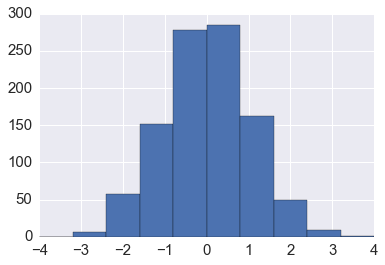
plt.hist(np.random.randn(1000), bins=np.linspace(-4,4,11))
pass
In [3]:
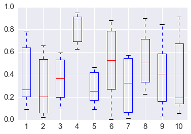
plt.boxplot(np.random.random((6,10)))
pass
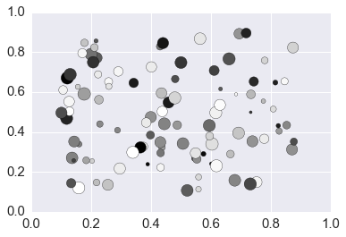
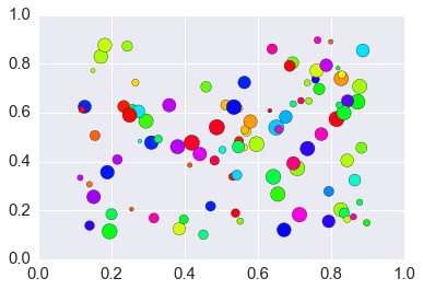
In [4]:
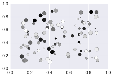
plt.scatter(*np.random.uniform(0.1, 0.9, (2,100)),
            s=np.random.randint(10, 200, 100),
            c=np.random.random(100))
pass
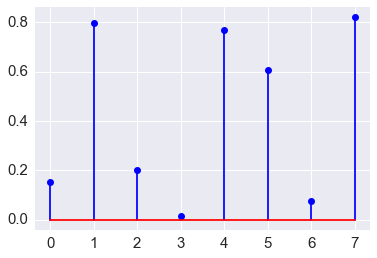
In [5]:
plt.stem(np.random.random(8))
plt.margins(0.05)
pass
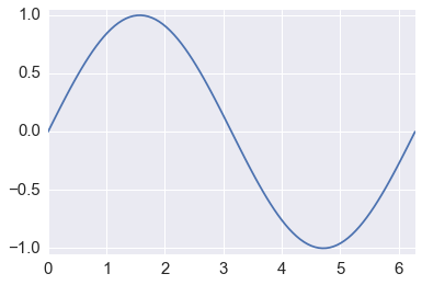
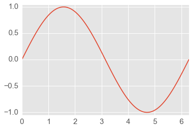
In [6]:
x = np.linspace(0, 2*np.pi, 100)
y = np.sin(x)
In [7]:
plt.plot(x, y)
plt.axis([0, 2*np.pi, -1.05, 1.05,])
pass
Colors
In [8]:
plt.scatter(*np.random.uniform(0.1, 0.9, (2,100)),
            s=np.random.randint(10, 200, 100),
            c=np.random.random(100))
pass
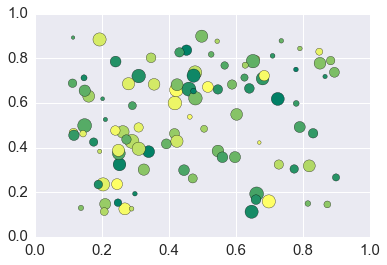
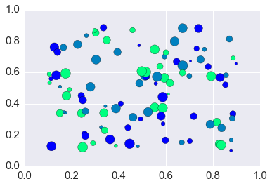
In [9]:
plt.scatter(*np.random.uniform(0.1, 0.9, (2,100)),
            s=np.random.randint(10, 200, 100),
            c=np.random.random(100), cmap='summer')
pass
In [10]:
plt.scatter(*np.random.uniform(0.1, 0.9, (2,100)),
            s=np.random.randint(10, 200, 100),
            c=np.random.random(100), cmap='hsv')
pass
Gettting a list of colors from a colormap
Giving an argument of 0.0 < x < 1.0 to a colormap gives the
appropriate interpolated color.
In [11]:
# find the bottom, middle and top colors of the winter colormap
colors = plt.cm.winter(np.linspace(0, 1, 3))
colors
Out[11]:
array([[ 0.        ,  0.        ,  1.        ,  1.        ],
       [ 0.        ,  0.50196078,  0.74901961,  1.        ],
       [ 0.        ,  1.        ,  0.5       ,  1.        ]])
In [12]:
plt.scatter(*np.random.uniform(0.1, 0.9, (2,100)),
            s=np.random.randint(10, 200, 100),
            c=colors)
pass
Styles
In [13]:
plt.style.available
Out[13]:
['seaborn-ticks',
 'seaborn-white',
 'seaborn-whitegrid',
 'seaborn-colorblind',
 'seaborn-pastel',
 'seaborn-poster',
 'seaborn-paper',
 'ggplot',
 'seaborn-deep',
 'bmh',
 'seaborn-talk',
 'seaborn-dark',
 'dark_background',
 'seaborn-bright',
 'fivethirtyeight',
 'seaborn-notebook',
 'classic',
 'presentation',
 'seaborn-muted',
 'seaborn-dark-palette',
 'grayscale',
 'seaborn-darkgrid']
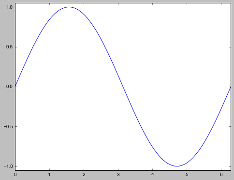
In [14]:
with plt.style.context('classic'):
    plt.plot(x, y)
    plt.axis([0, 2*np.pi, -1.05, 1.05,])
In [15]:
with plt.style.context('fivethirtyeight'):
    plt.plot(x, y)
    plt.axis([0, 2*np.pi, -1.05, 1.05,])
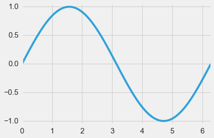
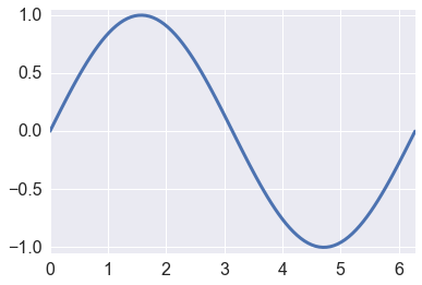
In [16]:
with plt.style.context('ggplot'):
    plt.plot(x, y)
    plt.axis([0, 2*np.pi, -1.05, 1.05,])
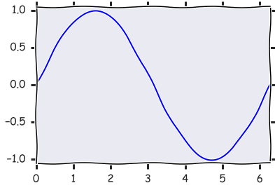
In [17]:
with plt.xkcd():
    plt.plot(x, y)
    plt.axis([0, 2*np.pi, -1.05, 1.05,])
Creating your onw style
Many, many options can be configured.
In [18]:
plt.rcParams
Out[18]:
RcParams({'agg.path.chunksize': 0,
          'animation.avconv_args': [],
          'animation.avconv_path': 'avconv',
          'animation.bitrate': -1,
          'animation.codec': 'mpeg4',
          'animation.convert_args': [],
          'animation.convert_path': 'convert',
          'animation.ffmpeg_args': [],
          'animation.ffmpeg_path': 'ffmpeg',
          'animation.frame_format': 'png',
          'animation.html': 'none',
          'animation.mencoder_args': [],
          'animation.mencoder_path': 'mencoder',
          'animation.writer': 'ffmpeg',
          'axes.axisbelow': True,
          'axes.edgecolor': 'white',
          'axes.facecolor': '#EAEAF2',
          'axes.formatter.limits': [-7, 7],
          'axes.formatter.use_locale': False,
          'axes.formatter.use_mathtext': False,
          'axes.formatter.useoffset': True,
          'axes.grid': True,
          'axes.grid.axis': 'both',
          'axes.grid.which': 'major',
          'axes.hold': True,
          'axes.labelcolor': '.15',
          'axes.labelpad': 5.0,
          'axes.labelsize': 16.5,
          'axes.labelweight': 'normal',
          'axes.linewidth': 0.0,
          'axes.prop_cycle': cycler('color', [(0.2980392156862745, 0.4470588235294118, 0.6901960784313725), (0.3333333333333333, 0.6588235294117647, 0.40784313725490196), (0.7686274509803922, 0.3058823529411765, 0.3215686274509804), (0.5058823529411764, 0.4470588235294118, 0.6980392156862745), (0.8, 0.7254901960784313, 0.4549019607843137), (0.39215686274509803, 0.7098039215686275, 0.803921568627451)]),
          'axes.spines.bottom': True,
          'axes.spines.left': True,
          'axes.spines.right': True,
          'axes.spines.top': True,
          'axes.titlesize': 18.0,
          'axes.titleweight': 'normal',
          'axes.unicode_minus': True,
          'axes.xmargin': 0.0,
          'axes.ymargin': 0.0,
          'axes3d.grid': True,
          'backend': 'module://ipykernel.pylab.backend_inline',
          'backend.qt4': 'PyQt4',
          'backend.qt5': 'PyQt5',
          'backend_fallback': True,
          'boxplot.bootstrap': None,
          'boxplot.boxprops.color': 'b',
          'boxplot.boxprops.linestyle': '-',
          'boxplot.boxprops.linewidth': 1.0,
          'boxplot.capprops.color': 'k',
          'boxplot.capprops.linestyle': '-',
          'boxplot.capprops.linewidth': 1.0,
          'boxplot.flierprops.color': 'b',
          'boxplot.flierprops.linestyle': 'none',
          'boxplot.flierprops.linewidth': 1.0,
          'boxplot.flierprops.marker': '+',
          'boxplot.flierprops.markeredgecolor': 'k',
          'boxplot.flierprops.markerfacecolor': 'b',
          'boxplot.flierprops.markersize': 6.0,
          'boxplot.meanline': False,
          'boxplot.meanprops.color': 'r',
          'boxplot.meanprops.linestyle': '-',
          'boxplot.meanprops.linewidth': 1.0,
          'boxplot.medianprops.color': 'r',
          'boxplot.medianprops.linestyle': '-',
          'boxplot.medianprops.linewidth': 1.0,
          'boxplot.notch': False,
          'boxplot.patchartist': False,
          'boxplot.showbox': True,
          'boxplot.showcaps': True,
          'boxplot.showfliers': True,
          'boxplot.showmeans': False,
          'boxplot.vertical': True,
          'boxplot.whiskerprops.color': 'b',
          'boxplot.whiskerprops.linestyle': '--',
          'boxplot.whiskerprops.linewidth': 1.0,
          'boxplot.whiskers': 1.5,
          'contour.corner_mask': True,
          'contour.negative_linestyle': 'dashed',
          'datapath': '/Users/cliburn/anaconda/envs/py35/lib/python3.5/site-packages/matplotlib/mpl-data',
          'docstring.hardcopy': False,
          'errorbar.capsize': 3.0,
          'examples.directory': '',
          'figure.autolayout': False,
          'figure.dpi': 80.0,
          'figure.edgecolor': (1, 1, 1, 0),
          'figure.facecolor': (1, 1, 1, 0),
          'figure.figsize': [6.0, 4.0],
          'figure.frameon': True,
          'figure.max_open_warning': 20,
          'figure.subplot.bottom': 0.125,
          'figure.subplot.hspace': 0.2,
          'figure.subplot.left': 0.125,
          'figure.subplot.right': 0.9,
          'figure.subplot.top': 0.9,
          'figure.subplot.wspace': 0.2,
          'figure.titlesize': 'medium',
          'figure.titleweight': 'normal',
          'font.cursive': ['Apple Chancery',
                           'Textile',
                           'Zapf Chancery',
                           'Sand',
                           'Script MT',
                           'Felipa',
                           'cursive'],
          'font.family': ['sans-serif'],
          'font.fantasy': ['Comic Sans MS',
                           'Chicago',
                           'Charcoal',
                           'ImpactWestern',
                           'Humor Sans',
                           'fantasy'],
          'font.monospace': ['Bitstream Vera Sans Mono',
                             'DejaVu Sans Mono',
                             'Andale Mono',
                             'Nimbus Mono L',
                             'Courier New',
                             'Courier',
                             'Fixed',
                             'Terminal',
                             'monospace'],
          'font.sans-serif': ['Arial',
                              'Liberation Sans',
                              'Bitstream Vera Sans',
                              'sans-serif'],
          'font.serif': ['Bitstream Vera Serif',
                         'DejaVu Serif',
                         'New Century Schoolbook',
                         'Century Schoolbook L',
                         'Utopia',
                         'ITC Bookman',
                         'Bookman',
                         'Nimbus Roman No9 L',
                         'Times New Roman',
                         'Times',
                         'Palatino',
                         'Charter',
                         'serif'],
          'font.size': 10.0,
          'font.stretch': 'normal',
          'font.style': 'normal',
          'font.variant': 'normal',
          'font.weight': 'normal',
          'grid.alpha': 1.0,
          'grid.color': 'white',
          'grid.linestyle': '-',
          'grid.linewidth': 1.0,
          'image.aspect': 'equal',
          'image.cmap': 'Greys',
          'image.composite_image': True,
          'image.interpolation': 'bilinear',
          'image.lut': 256,
          'image.origin': 'upper',
          'image.resample': False,
          'interactive': True,
          'keymap.all_axes': ['a'],
          'keymap.back': ['left', 'c', 'backspace'],
          'keymap.forward': ['right', 'v'],
          'keymap.fullscreen': ['f', 'ctrl+f'],
          'keymap.grid': ['g'],
          'keymap.home': ['h', 'r', 'home'],
          'keymap.pan': ['p'],
          'keymap.quit': ['ctrl+w', 'cmd+w'],
          'keymap.save': ['s', 'ctrl+s'],
          'keymap.xscale': ['k', 'L'],
          'keymap.yscale': ['l'],
          'keymap.zoom': ['o'],
          'legend.borderaxespad': 0.5,
          'legend.borderpad': 0.4,
          'legend.columnspacing': 2.0,
          'legend.edgecolor': 'inherit',
          'legend.facecolor': 'inherit',
          'legend.fancybox': False,
          'legend.fontsize': 15.0,
          'legend.framealpha': None,
          'legend.frameon': False,
          'legend.handleheight': 0.7,
          'legend.handlelength': 2.0,
          'legend.handletextpad': 0.8,
          'legend.isaxes': True,
          'legend.labelspacing': 0.5,
          'legend.loc': 'upper right',
          'legend.markerscale': 1.0,
          'legend.numpoints': 1,
          'legend.scatterpoints': 1,
          'legend.shadow': False,
          'lines.antialiased': True,
          'lines.color': 'b',
          'lines.dash_capstyle': 'butt',
          'lines.dash_joinstyle': 'round',
          'lines.linestyle': '-',
          'lines.linewidth': 1.75,
          'lines.marker': 'None',
          'lines.markeredgewidth': 0.0,
          'lines.markersize': 7.0,
          'lines.solid_capstyle': 'round',
          'lines.solid_joinstyle': 'round',
          'markers.fillstyle': 'full',
          'mathtext.bf': 'serif:bold',
          'mathtext.cal': 'cursive',
          'mathtext.default': 'it',
          'mathtext.fallback_to_cm': True,
          'mathtext.fontset': 'cm',
          'mathtext.it': 'serif:italic',
          'mathtext.rm': 'serif',
          'mathtext.sf': 'sans\\-serif',
          'mathtext.tt': 'monospace',
          'nbagg.transparent': True,
          'patch.antialiased': True,
          'patch.edgecolor': 'k',
          'patch.facecolor': (0.2980392156862745,
                              0.4470588235294118,
                              0.6901960784313725),
          'patch.linewidth': 0.3,
          'path.effects': [],
          'path.simplify': True,
          'path.simplify_threshold': 0.1111111111111111,
          'path.sketch': None,
          'path.snap': True,
          'pdf.compression': 6,
          'pdf.fonttype': 3,
          'pdf.inheritcolor': False,
          'pdf.use14corefonts': False,
          'pgf.debug': False,
          'pgf.preamble': [],
          'pgf.rcfonts': True,
          'pgf.texsystem': 'xelatex',
          'plugins.directory': '.matplotlib_plugins',
          'polaraxes.grid': True,
          'ps.distiller.res': 6000,
          'ps.fonttype': 3,
          'ps.papersize': 'letter',
          'ps.useafm': False,
          'ps.usedistiller': False,
          'savefig.bbox': None,
          'savefig.directory': '~',
          'savefig.dpi': 72.0,
          'savefig.edgecolor': 'w',
          'savefig.facecolor': 'w',
          'savefig.format': 'png',
          'savefig.frameon': True,
          'savefig.jpeg_quality': 95,
          'savefig.orientation': 'portrait',
          'savefig.pad_inches': 0.1,
          'savefig.transparent': False,
          'svg.fonttype': 'path',
          'svg.image_inline': True,
          'svg.image_noscale': False,
          'text.antialiased': True,
          'text.color': '.15',
          'text.dvipnghack': None,
          'text.hinting': 'auto',
          'text.hinting_factor': 8,
          'text.latex.preamble': [],
          'text.latex.preview': False,
          'text.latex.unicode': False,
          'text.usetex': False,
          'timezone': 'UTC',
          'tk.window_focus': False,
          'toolbar': 'toolbar2',
          'verbose.fileo': 'sys.stdout',
          'verbose.level': 'silent',
          'webagg.open_in_browser': True,
          'webagg.port': 8988,
          'webagg.port_retries': 50,
          'xtick.color': '.15',
          'xtick.direction': 'out',
          'xtick.labelsize': 15.0,
          'xtick.major.pad': 7.0,
          'xtick.major.size': 0.0,
          'xtick.major.width': 1.0,
          'xtick.minor.pad': 4.0,
          'xtick.minor.size': 0.0,
          'xtick.minor.visible': False,
          'xtick.minor.width': 0.5,
          'ytick.color': '.15',
          'ytick.direction': 'out',
          'ytick.labelsize': 15.0,
          'ytick.major.pad': 7.0,
          'ytick.major.size': 0.0,
          'ytick.major.width': 1.0,
          'ytick.minor.pad': 4.0,
          'ytick.minor.size': 0.0,
          'ytick.minor.visible': False,
          'ytick.minor.width': 0.5})
In [19]:
%%file foo.mplstyle
axes.grid: True
axes.titlesize : 24
axes.labelsize : 20
lines.linewidth : 3
lines.markersize : 10
xtick.labelsize : 16
ytick.labelsize : 16
Overwriting foo.mplstyle
In [20]:
with plt.style.context('foo.mplstyle'):
    plt.plot(x, y)
    plt.axis([0, 2*np.pi, -1.05, 1.05,])
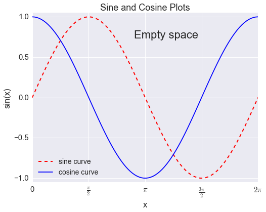
Customizing plots
In [21]:
plt.rcParams.update({'font.size': 22})

fig = plt.figure(figsize=(8,6))
ax = plt.subplot(1,1,1)
plt.plot(x, y, color='red', linewidth=2, linestyle='dashed', label='sine curve')
plt.plot(x, np.cos(x), 'b-', label='cosine curve')
plt.legend(loc='best', fontsize=14)
plt.axis([0, 2*np.pi, -1.05, 1.05,])
plt.xlabel('x')
plt.ylabel('sin(x)')
plt.xticks([0,0.5*np.pi,np.pi,1.5*np.pi,2*np.pi],
           [0, r'$\frac{\pi}{2}$', r'$\pi$', r'$\frac{3\pi}{2}$', r'$2\pi$'])
plt.title('Sine and Cosine Plots')
plt.text(0.45, 0.9, 'Empty space', transform=ax.transAxes, ha='left', va='top')
pass
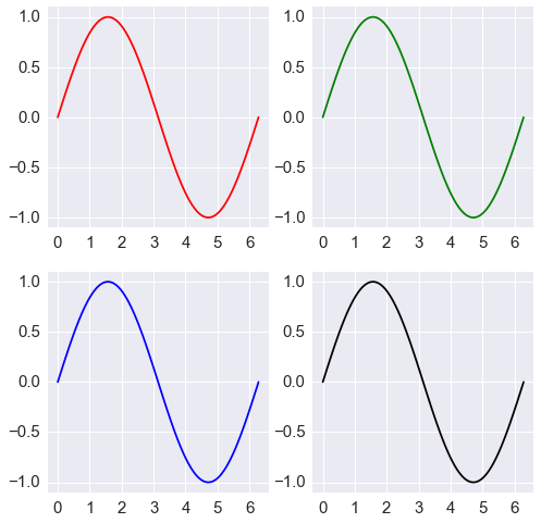
Plot layouts
In [22]:
fig, axes = plt.subplots(2,2,figsize=(8,8))
axes[0,0].plot(x,y, 'r')
axes[0,1].plot(x,y, 'g')
axes[1,0].plot(x,y, 'b')
axes[1,1].plot(x,y, 'k')
for ax in axes.ravel():
    ax.margins(0.05)
pass
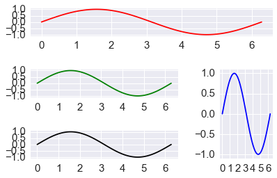
In [23]:
ax1 = plt.subplot2grid((3,3), (0,0), colspan=3)
ax2 = plt.subplot2grid((3,3), (1,0), colspan=2)
ax3 = plt.subplot2grid((3,3), (1,2), rowspan=2)
ax4 = plt.subplot2grid((3,3), (2,0), colspan=2)
axes = [ax1, ax2, ax3, ax4]
colors = ['r', 'g', 'b', 'k']
for ax, c in zip(axes, colors):
    ax.plot(x, y, c)
    ax.margins(0.05)
plt.tight_layout()
Seaborn
In [24]:
sns.set_context("notebook", font_scale=1.5, rc={"lines.linewidth": 2.5})
In [25]:
import numpy.random as rng
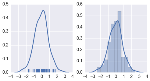
Density plots
In [26]:
xs = rng.normal(0,1,100)

fig, axes = plt.subplots(1, 2, figsize=(8,4))
sns.distplot(xs, hist=False, rug=True, ax=axes[0]);
sns.distplot(xs, hist=True, ax=axes[1])
pass
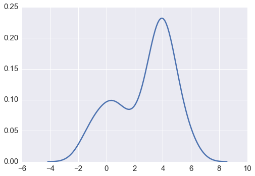
Kernel density estimate
In [27]:
sns.kdeplot(np.r_[rng.normal(0,1,50), rng.normal(4,0.8,100)])
pass
In [28]:
iris = sns.load_dataset('iris')
In [29]:
iris.head()
Out[29]:
| sepal_length | sepal_width | petal_length | petal_width | species | |
|---|---|---|---|---|---|
| 0 | 5.1 | 3.5 | 1.4 | 0.2 | setosa |
| 1 | 4.9 | 3.0 | 1.4 | 0.2 | setosa |
| 2 | 4.7 | 3.2 | 1.3 | 0.2 | setosa |
| 3 | 4.6 | 3.1 | 1.5 | 0.2 | setosa |
| 4 | 5.0 | 3.6 | 1.4 | 0.2 | setosa |
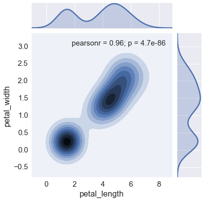
Joint distribution plot
In [30]:
sns.jointplot(x='petal_length', y='petal_width', data=iris, kind='kdeplot')
pass
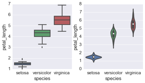
Box and violin plots
In [31]:
fig, axes = plt.subplots(1, 2, figsize=(8,4))

sns.boxplot(x='species', y='petal_length', data=iris, ax=axes[0])
sns.violinplot(x='species', y='petal_length', data=iris, ax=axes[1])
pass
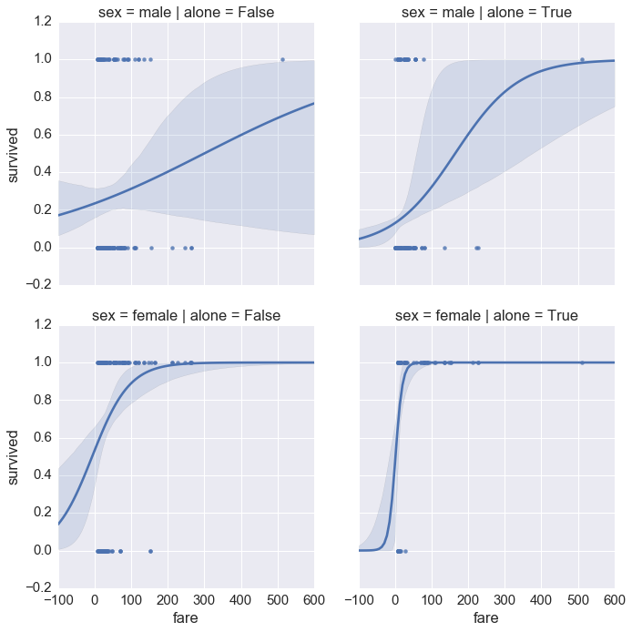
Composite plots
In [32]:
url = 'https://raw.githubusercontent.com/mwaskom/seaborn-data/master/titanic.csv'
titanic = pd.read_csv(url)
In [33]:
titanic.head()
Out[33]:
| survived | pclass | sex | age | sibsp | parch | fare | embarked | class | who | adult_male | deck | embark_town | alive | alone | |
|---|---|---|---|---|---|---|---|---|---|---|---|---|---|---|---|
| 0 | 0 | 3 | male | 22 | 1 | 0 | 7.2500 | S | Third | man | True | NaN | Southampton | no | False |
| 1 | 1 | 1 | female | 38 | 1 | 0 | 71.2833 | C | First | woman | False | C | Cherbourg | yes | False |
| 2 | 1 | 3 | female | 26 | 0 | 0 | 7.9250 | S | Third | woman | False | NaN | Southampton | yes | True |
| 3 | 1 | 1 | female | 35 | 1 | 0 | 53.1000 | S | First | woman | False | C | Southampton | yes | False |
| 4 | 0 | 3 | male | 35 | 0 | 0 | 8.0500 | S | Third | man | True | NaN | Southampton | no | True |
In [34]:
sns.set_context('notebook', font_scale=1.5)
In [35]:
sns.lmplot(x='fare', y='survived', col='alone', row='sex', data=titanic, logistic=True)
pass
In [36]:
g = sns.PairGrid(titanic,
                 y_vars=['fare', 'age'],
                 x_vars=['sex', 'class', 'embark_town' ],
                 aspect=1, size=5.5)
g.map(sns.stripplot, jitter=True, palette="bright")
pass

Using ggplot as an alternative to seaborn.
The ggplot module is a port of R’s ggplot2 - usage is very
similar except for the following minor differences:
- Pass in a
pandasdataframe - aethetics comes before data in the argument list ot ggplot
- Give column names and other arugments (e.g.. function to call) as strings
- You need to use the line continuation character
\to extend over multiple lines
Only the most elementary examples are shown below. The ggplot module
is extremely rich and sophisticated with a steep learning curve if
you’re not already familiar with it from R. Please see
documentation for
details.
In [37]:
from ggplot import *
Interacting with R
In [38]:
%load_ext rpy2.ipython
Note that we are exporting the R mtcars dataframe to Python (converts to pandas DataFrame)
In [39]:
%R -o mtcars
In [40]:
mtcars.head()
Out[40]:
| mpg | cyl | disp | hp | drat | wt | qsec | vs | am | gear | carb | |
|---|---|---|---|---|---|---|---|---|---|---|---|
| Mazda RX4 | 21.0 | 6 | 160 | 110 | 3.90 | 2.620 | 16.46 | 0 | 1 | 4 | 4 |
| Mazda RX4 Wag | 21.0 | 6 | 160 | 110 | 3.90 | 2.875 | 17.02 | 0 | 1 | 4 | 4 |
| Datsun 710 | 22.8 | 4 | 108 | 93 | 3.85 | 2.320 | 18.61 | 1 | 1 | 4 | 1 |
| Hornet 4 Drive | 21.4 | 6 | 258 | 110 | 3.08 | 3.215 | 19.44 | 1 | 0 | 3 | 1 |
| Hornet Sportabout | 18.7 | 8 | 360 | 175 | 3.15 | 3.440 | 17.02 | 0 | 0 | 3 | 2 |
In [41]:
ggplot(aes(x='wt', y='mpg'), data=mtcars,) + geom_point()
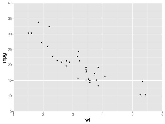
Out[41]:
<ggplot: (292414163)>
In [42]:
ggplot(aes(x='wt', y='mpg'), data=mtcars) + geom_point() + geom_smooth(method='loess')
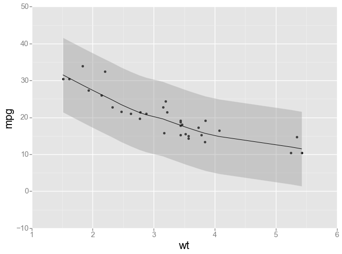
Out[42]:
<ggplot: (292201757)>
In [43]:
ggplot(aes(x='wt', y='mpg'), data=mtcars) + geom_point() + geom_line()
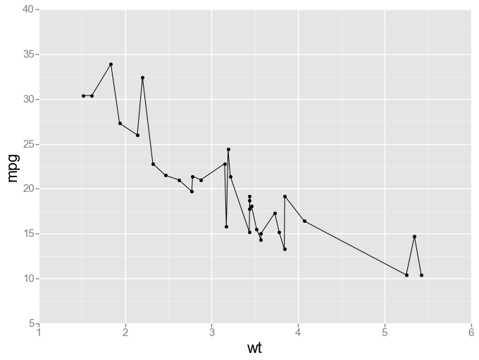
Out[43]:
<ggplot: (287265863)>
In [44]:
ggplot(aes(x='mpg'), data=mtcars) + geom_histogram(binwidth=2)
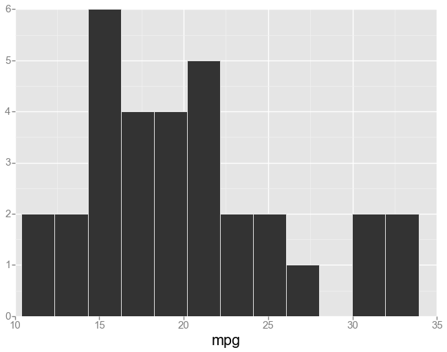
Out[44]:
<ggplot: (-9223372036566578744)>
In [45]:
ggplot(aes(x='mpg'), mtcars) + \
geom_line(stat="density") + \
xlim(2.97, 41.33) + \
labs(title="Density plot")
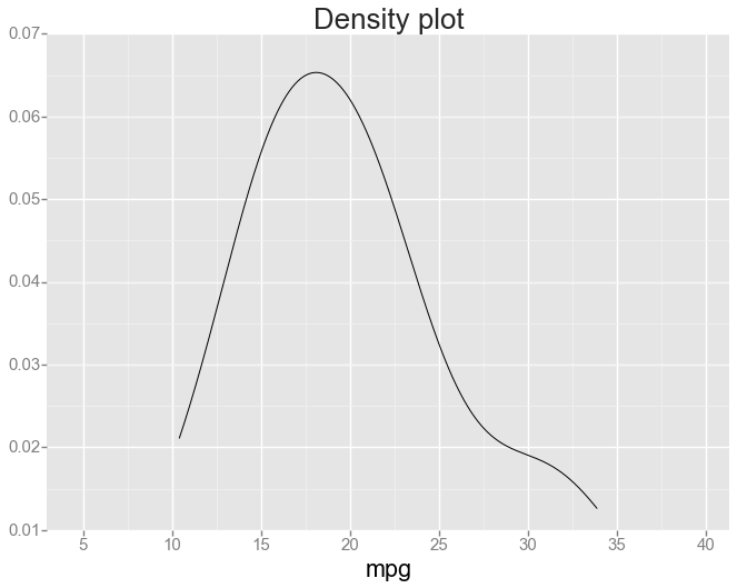
Out[45]:
<ggplot: (288465612)>
Use ggplot in R directly with %R magic
In [46]:
cars = mtcars
Note that we pass in Python variables with the -i optin and using the %%R cell magic
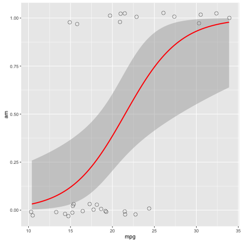
In [52]:
%%R -i cars
library('ggplot2')
ggplot(cars, aes(x=mpg, y=am)) +
geom_point(position=position_jitter(width=.3, height=.08), shape=21, alpha=0.6, size=3) +
stat_smooth(method=glm, method.args=list(family="binomial"), color="red")