Basic plots with matplotlib
In [1]:
import numpy as np
import matplotlib.pyplot as plt
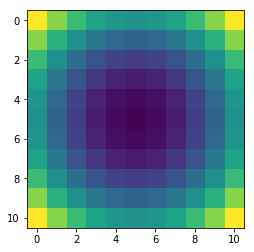
Displaying matrices
In [2]:
img = np.fromfunction(lambda i, j:  (i-5)**2 + (j-5)**2,
                      (11,11))
In [3]:
g = plt.imshow(img, interpolation='nearest')
In [4]:
plt.show()

To set display on by default
In [5]:
%matplotlib inline
In [6]:
g = plt.imshow(img, interpolation='nearest')
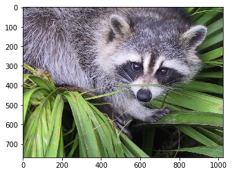
Images as arrays
In [7]:
from scipy import misc
face = misc.imread('figs/face.png')
In [8]:
face.shape
Out[8]:
(768, 1024, 3)
In [9]:
face
Out[9]:
array([[[121, 112, 131],
        [138, 129, 148],
        [153, 144, 165],
        ...,
        [119, 126,  74],
        [131, 136,  82],
        [139, 144,  90]],

       [[ 89,  82, 100],
        [110, 103, 121],
        [130, 122, 143],
        ...,
        [118, 125,  71],
        [134, 141,  87],
        [146, 153,  99]],

       [[ 73,  66,  84],
        [ 94,  87, 105],
        [115, 108, 126],
        ...,
        [117, 126,  71],
        [133, 142,  87],
        [144, 153,  98]],

       ...,
       [[ 87, 106,  76],
        [ 94, 110,  81],
        [107, 124,  92],
        ...,
        [120, 158,  97],
        [119, 157,  96],
        [119, 158,  95]],

       [[ 85, 101,  72],
        [ 95, 111,  82],
        [112, 127,  96],
        ...,
        [121, 157,  96],
        [120, 156,  94],
        [120, 156,  94]],

       [[ 85, 101,  74],
        [ 97, 113,  84],
        [111, 126,  97],
        ...,
        [120, 156,  95],
        [119, 155,  93],
        [118, 154,  92]]], dtype=uint8)
In [10]:
plt.imshow(face);
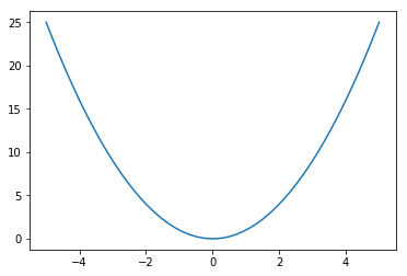
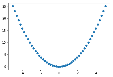
Line plots
In [11]:
x = np.linspace(-5, 5, 50)
y = x**2
In [12]:
plt.plot(x, y);
In [13]:
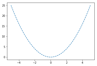
plt.plot(x, y, '--');

In [14]:
plt.plot(x, y, linestyle='dashed');
In [15]:
plt.plot(x, y, 'o');
In [16]:
plt.plot(x, y, marker='o', markersize=5, color='salmon',
         linestyle='solid',);

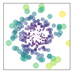
Scatter plots
In [17]:
x = np.random.multivariate_normal(np.zeros(2), np.eye(2), 250)
v = 50*(x**2).sum(1)

plt.scatter(x[:,0], x[:,1], s=v, c=v, alpha=0.5)
plt.axis('square');
plt.axis([-3,3,-3,3])
plt.xticks([])
plt.yticks([]);
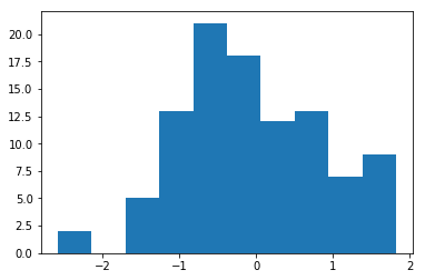
Histograms
In [18]:
x = np.random.randn(100)
In [19]:
plt.hist(x);
In [20]:
for i in range(5):
    x = np.random.normal(i, 1, 100)
    plt.hist(x, bins=15, alpha=0.5, normed=True);

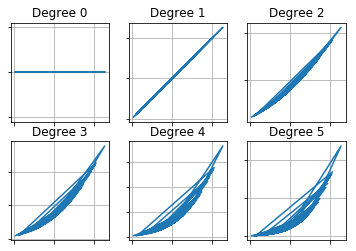
Multiple plots
In [21]:
nrows = 2
ncols = 3
fig, axes = plt.subplots(nrows, ncols, figsize=(ncols*2, nrows*2))
for i, ax in enumerate(axes.ravel()):
    ax.plot(x, x**i)
    ax.grid(True)
    ax.set_xticklabels([])
    ax.set_yticklabels([])
    ax.set_title('Degree {}'.format(i))
Styles
In [22]:
x = np.linspace(-5, 5, 50)
y = x**2
In [23]:
plt.style.available
Out[23]:
['_classic_test',
 'bmh',
 'classic',
 'dark_background',
 'fivethirtyeight',
 'ggplot',
 'grayscale',
 'seaborn-bright',
 'seaborn-colorblind',
 'seaborn-dark-palette',
 'seaborn-dark',
 'seaborn-darkgrid',
 'seaborn-deep',
 'seaborn-muted',
 'seaborn-notebook',
 'seaborn-paper',
 'seaborn-pastel',
 'seaborn-poster',
 'seaborn-talk',
 'seaborn-ticks',
 'seaborn-white',
 'seaborn-whitegrid',
 'seaborn']
In [24]:
with plt.style.context('ggplot'):
    plt.plot(x, y);

In [25]:
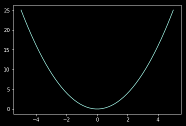
with plt.style.context('dark_background'):
    plt.plot(x, y);
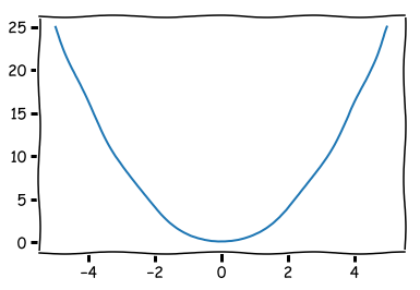
In [26]:
with plt.xkcd():
    plt.plot(x, y);
In [ ]: