Pandas Part 2
Part 1 assumed that the data.frame is in a tidy format, with one
observation per row and one variable per column. Real-world data is
often not so obliging, and we have to clean and wrangle it before we can
analyze the data efficiently.
Data cleaning operations
- Move column to index
- Move index to column
- Rearranging column order
- Change or rename values in the table
- Dealing with missing data
- Dealing with duplicate data
Special operations (strings and categorical variables)
- Splitting single string column into multiple columns
- Joining multiple string columns into single column
- Creating dummy variables from categorical variables for regression or
machine learning
Data wrangling (Generally involve changes of shapes)
- Moving data from multiple columns to single column (melt)
- Moving multiple categories in a column to separate columns (pivot)
- Pivoting with aggregation (pivot_table)
- Combining multiple data frames
Data cleaning
Swapping columns and indexes
|
age |
pid |
wt |
| 0 |
23 |
101 |
150 |
| 1 |
34 |
102 |
160 |
| 2 |
45 |
103 |
170 |
|
age |
wt |
| pid |
|
|
| 101 |
23 |
150 |
| 102 |
34 |
160 |
| 103 |
45 |
170 |
|
pid |
age |
wt |
| 0 |
101 |
23 |
150 |
| 1 |
102 |
34 |
160 |
| 2 |
103 |
45 |
170 |
Explicit replacement
|
age |
pid |
wt |
| 0 |
young |
101 |
150 |
| 1 |
old |
102 |
160 |
| 2 |
old |
103 |
170 |
Missing data
|
mon |
tue |
wed |
| pid |
|
|
|
| 101 |
10.0 |
11.0 |
12.0 |
| 102 |
11.0 |
NaN |
13.0 |
| 103 |
NaN |
NaN |
10.0 |
| 104 |
NaN |
NaN |
NaN |
|
mon |
tue |
wed |
| pid |
|
|
|
| 101 |
False |
False |
False |
| 102 |
False |
True |
False |
| 103 |
True |
True |
False |
| 104 |
True |
True |
True |
|
mon |
tue |
wed |
| pid |
|
|
|
| 101 |
True |
True |
True |
| 102 |
True |
False |
True |
| 103 |
False |
False |
True |
| 104 |
False |
False |
False |
Drop any row containing missing data
|
mon |
tue |
wed |
| pid |
|
|
|
| 101 |
10.0 |
11.0 |
12.0 |
Drop only rows where all data is missing
|
mon |
tue |
wed |
| pid |
|
|
|
| 101 |
10.0 |
11.0 |
12.0 |
| 102 |
11.0 |
NaN |
13.0 |
| 103 |
NaN |
NaN |
10.0 |
Drop any column with missing data
|
wed |
| pid |
|
| 101 |
12.0 |
| 102 |
13.0 |
| 103 |
10.0 |
Simple imputation
|
mon |
tue |
wed |
| pid |
|
|
|
| 101 |
10.0 |
11.0 |
12.0 |
| 102 |
11.0 |
NaN |
13.0 |
| 103 |
NaN |
NaN |
10.0 |
| 104 |
NaN |
NaN |
NaN |
Fill with column mean
|
mon |
tue |
wed |
| pid |
|
|
|
| 101 |
10.0 |
11.0 |
12.000000 |
| 102 |
11.0 |
11.0 |
13.000000 |
| 103 |
10.5 |
11.0 |
10.000000 |
| 104 |
10.5 |
11.0 |
11.666667 |
Fill wiht specific values
|
mon |
tue |
wed |
| pid |
|
|
|
| 101 |
10.0 |
11.0 |
12.0 |
| 102 |
11.0 |
0.0 |
13.0 |
| 103 |
0.0 |
0.0 |
10.0 |
| 104 |
0.0 |
0.0 |
0.0 |
|
mon |
tue |
wed |
| pid |
|
|
|
| 101 |
10.0 |
11.0 |
12.0 |
| 102 |
11.0 |
11.0 |
13.0 |
| 103 |
10.0 |
11.0 |
10.0 |
| 104 |
10.0 |
11.0 |
12.0 |
Duplicate data
|
pid |
mon |
tue |
wed |
| 0 |
101 |
10 |
11 |
12 |
| 1 |
102 |
11 |
12 |
13 |
| 2 |
103 |
10 |
10 |
10 |
| 3 |
102 |
11 |
12 |
13 |
| 4 |
102 |
10 |
11 |
14 |
| 5 |
101 |
10 |
11 |
12 |
0    False
1    False
2    False
3     True
4    False
5     True
dtype: bool
0    False
1    False
2    False
3     True
4     True
5     True
dtype: bool
|
pid |
mon |
tue |
wed |
| 0 |
101 |
10 |
11 |
12 |
| 1 |
102 |
11 |
12 |
13 |
| 2 |
103 |
10 |
10 |
10 |
| 4 |
102 |
10 |
11 |
14 |
|
pid |
mon |
tue |
wed |
| 0 |
101 |
10 |
11 |
12 |
| 1 |
102 |
11 |
12 |
13 |
| 2 |
103 |
10 |
10 |
10 |
Special operations on strings and factors
Strings
|
id |
mon |
tue |
wed |
| 0 |
101:duke:2017 |
10 |
11 |
12 |
| 1 |
102:duke:2017 |
11 |
12 |
13 |
| 2 |
103:duke:2017 |
10 |
10 |
10 |
| 3 |
102:unc:2016 |
11 |
12 |
13 |
| 4 |
102:unc:2017 |
10 |
11 |
14 |
| 5 |
101:unc:2017 |
10 |
11 |
12 |
0    [101, duke, 2017]
1    [102, duke, 2017]
2    [103, duke, 2017]
3     [102, unc, 2016]
4     [102, unc, 2017]
5     [101, unc, 2017]
Name: id, dtype: object
0    2017
1    2017
2    2017
3    2016
4    2017
5    2017
Name: id, dtype: object
|
id |
mon |
tue |
wed |
pid |
site |
year |
| 0 |
101:duke:2017 |
10 |
11 |
12 |
101 |
duke |
2017 |
| 1 |
102:duke:2017 |
11 |
12 |
13 |
102 |
duke |
2017 |
| 2 |
103:duke:2017 |
10 |
10 |
10 |
103 |
duke |
2017 |
| 3 |
102:unc:2016 |
11 |
12 |
13 |
102 |
unc |
2016 |
| 4 |
102:unc:2017 |
10 |
11 |
14 |
102 |
unc |
2017 |
| 5 |
101:unc:2017 |
10 |
11 |
12 |
101 |
unc |
2017 |
Rearrange and drop old id column
|
pid |
site |
year |
mon |
tue |
wed |
| 0 |
101 |
duke |
2017 |
10 |
11 |
12 |
| 1 |
102 |
duke |
2017 |
11 |
12 |
13 |
| 2 |
103 |
duke |
2017 |
10 |
10 |
10 |
| 3 |
102 |
unc |
2016 |
11 |
12 |
13 |
| 4 |
102 |
unc |
2017 |
10 |
11 |
14 |
| 5 |
101 |
unc |
2017 |
10 |
11 |
12 |
|
0 |
1 |
| 0 |
duke |
2017 |
| 1 |
duke |
2017 |
| 2 |
duke |
2017 |
| 3 |
unc |
2016 |
| 4 |
unc |
2017 |
| 5 |
unc |
2017 |
|
id |
mon |
tue |
wed |
pid |
site |
year |
| 3 |
102:unc:2016 |
11 |
12 |
13 |
102 |
unc |
2016 |
| 4 |
102:unc:2017 |
10 |
11 |
14 |
102 |
unc |
2017 |
| 5 |
101:unc:2017 |
10 |
11 |
12 |
101 |
unc |
2017 |
Joining multiple string columns
0    101:duke:2017
1    102:duke:2017
2    103:duke:2017
3     102:unc:2016
4     102:unc:2017
5     101:unc:2017
dtype: object
Another method if you are combining LOTS of columns
0    101:duke:2017
1    102:duke:2017
2    103:duke:2017
3     102:unc:2016
4     102:unc:2017
5     101:unc:2017
dtype: object
Categorical variables
|
pid |
site |
year |
mon |
tue |
wed |
| 0 |
101 |
duke |
2017 |
10 |
11 |
12 |
| 1 |
102 |
duke |
2017 |
11 |
12 |
13 |
| 2 |
103 |
duke |
2017 |
10 |
10 |
10 |
| 3 |
102 |
unc |
2016 |
11 |
12 |
13 |
| 4 |
102 |
unc |
2017 |
10 |
11 |
14 |
| 5 |
101 |
unc |
2017 |
10 |
11 |
12 |
0    duke
1    duke
2    duke
3     unc
4     unc
5     unc
Name: site, dtype: category
Categories (2, object): [duke, unc]
0    0
1    0
2    0
3    1
4    1
5    1
dtype: int8
Index(['duke', 'unc'], dtype='object')
0    duke
1    duke
2    duke
3     unc
4     unc
5     unc
Name: site, dtype: category
Categories (2, object): [unc < duke]
One-hot encoding
For regression models, it is often necessary to convert a single column
of categorical variables into dummy variable, with one dummy variable
for each possible category. In machine learning applications, this is
known as one-hot encoding.
|
race |
vals |
| 0 |
brown |
0.260416 |
| 1 |
white |
0.079823 |
| 2 |
black |
0.912978 |
| 3 |
black |
0.711759 |
| 4 |
white |
0.059453 |
| 5 |
brown |
0.024857 |
| 6 |
white |
0.960330 |
| 7 |
brown |
0.870268 |
| 8 |
yellow |
0.008312 |
| 9 |
brown |
0.345326 |
0     brown
1     white
2     black
3     black
4     white
5     brown
6     white
7     brown
8    yellow
9     brown
Name: race, dtype: category
Categories (4, object): [black, brown, white, yellow]
|
black |
brown |
white |
yellow |
| 0 |
0 |
1 |
0 |
0 |
| 1 |
0 |
0 |
1 |
0 |
| 2 |
1 |
0 |
0 |
0 |
| 3 |
1 |
0 |
0 |
0 |
| 4 |
0 |
0 |
1 |
0 |
| 5 |
0 |
1 |
0 |
0 |
| 6 |
0 |
0 |
1 |
0 |
| 7 |
0 |
1 |
0 |
0 |
| 8 |
0 |
0 |
0 |
1 |
| 9 |
0 |
1 |
0 |
0 |
|
race |
vals |
black |
brown |
white |
yellow |
| 0 |
brown |
0.260416 |
0 |
1 |
0 |
0 |
| 1 |
white |
0.079823 |
0 |
0 |
1 |
0 |
| 2 |
black |
0.912978 |
1 |
0 |
0 |
0 |
| 3 |
black |
0.711759 |
1 |
0 |
0 |
0 |
| 4 |
white |
0.059453 |
0 |
0 |
1 |
0 |
| 5 |
brown |
0.024857 |
0 |
1 |
0 |
0 |
| 6 |
white |
0.960330 |
0 |
0 |
1 |
0 |
| 7 |
brown |
0.870268 |
0 |
1 |
0 |
0 |
| 8 |
yellow |
0.008312 |
0 |
0 |
0 |
1 |
| 9 |
brown |
0.345326 |
0 |
1 |
0 |
0 |
Data Wrangling
Hierarchical indexing
|
|
weight |
| women |
pregnancy |
|
| anne |
1 |
8.661477 |
| 2 |
6.524455 |
| 3 |
7.052574 |
| bella |
1 |
7.183759 |
| 2 |
7.095648 |
| 3 |
9.075680 |
| carrie |
1 |
6.659004 |
| 2 |
8.807852 |
MultiIndex(levels=[['anne', 'bella', 'carrie'], [1, 2, 3]],
           labels=[[0, 0, 0, 1, 1, 1, 2, 2], [0, 1, 2, 0, 1, 2, 0, 1]],
           names=['women', 'pregnancy'])
Swapping levels
|
|
weight |
| pregnancy |
women |
|
| 1 |
anne |
8.661477 |
| bella |
7.183759 |
| carrie |
6.659004 |
| 2 |
anne |
6.524455 |
| bella |
7.095648 |
| carrie |
8.807852 |
| 3 |
anne |
7.052574 |
| bella |
9.075680 |
Partial indexing
|
weight |
| pregnancy |
|
| 1 |
7.183759 |
| 2 |
7.095648 |
| 3 |
9.075680 |
Unstack
This rotates from the rows to the columns.
|
weight |
| women |
anne |
bella |
carrie |
| pregnancy |
|
|
|
| 1 |
8.661477 |
7.183759 |
6.659004 |
| 2 |
6.524455 |
7.095648 |
8.807852 |
| 3 |
7.052574 |
9.075680 |
NaN |
|
weight |
| pregnancy |
1 |
2 |
3 |
| women |
|
|
|
| anne |
8.661477 |
6.524455 |
7.052574 |
| bella |
7.183759 |
7.095648 |
9.075680 |
| carrie |
6.659004 |
8.807852 |
NaN |
Stack
This rotates from the columns to the rows
|
weight |
| women |
anne |
bella |
carrie |
| pregnancy |
|
|
|
| 1 |
8.661477 |
7.183759 |
6.659004 |
| 2 |
6.524455 |
7.095648 |
8.807852 |
| 3 |
7.052574 |
9.075680 |
NaN |
|
women |
anne |
bella |
carrie |
| pregnancy |
|
|
|
|
| 1 |
weight |
8.661477 |
7.183759 |
6.659004 |
| 2 |
weight |
6.524455 |
7.095648 |
8.807852 |
| 3 |
weight |
7.052574 |
9.075680 |
NaN |
|
|
weight |
| pregnancy |
women |
|
| 1 |
anne |
8.661477 |
| bella |
7.183759 |
| carrie |
6.659004 |
| 2 |
anne |
6.524455 |
| bella |
7.095648 |
| carrie |
8.807852 |
| 3 |
anne |
7.052574 |
| bella |
9.075680 |
“Flattening” a hierarchical index
|
women |
pregnancy |
weight |
| 0 |
anne |
1 |
8.661477 |
| 1 |
anne |
2 |
6.524455 |
| 2 |
anne |
3 |
7.052574 |
| 3 |
bella |
1 |
7.183759 |
| 4 |
bella |
2 |
7.095648 |
| 5 |
bella |
3 |
9.075680 |
| 6 |
carrie |
1 |
6.659004 |
| 7 |
carrie |
2 |
8.807852 |
|
women |
weight |
| pregnancy |
|
|
| 1 |
anne |
8.661477 |
| 2 |
anne |
6.524455 |
| 3 |
anne |
7.052574 |
| 1 |
bella |
7.183759 |
| 2 |
bella |
7.095648 |
| 3 |
bella |
9.075680 |
| 1 |
carrie |
6.659004 |
| 2 |
carrie |
8.807852 |
Summary by level
|
|
weight |
| women |
pregnancy |
|
| anne |
1 |
8.661477 |
| 2 |
6.524455 |
| 3 |
7.052574 |
| bella |
1 |
7.183759 |
| 2 |
7.095648 |
| 3 |
9.075680 |
| carrie |
1 |
6.659004 |
| 2 |
8.807852 |
|
weight |
| women |
|
| anne |
7.412835 |
| bella |
7.785029 |
| carrie |
7.733428 |
|
weight |
| pregnancy |
|
| 1 |
7.501413 |
| 2 |
7.475985 |
| 3 |
8.064127 |
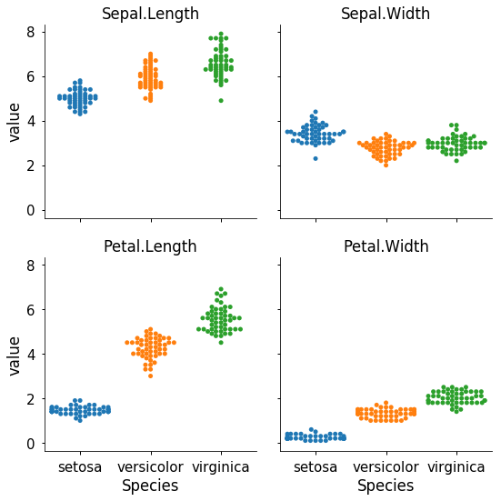
Reshape and pivot data
|
Sepal.Length |
Sepal.Width |
Petal.Length |
Petal.Width |
Species |
| 1 |
5.1 |
3.5 |
1.4 |
0.2 |
setosa |
| 2 |
4.9 |
3.0 |
1.4 |
0.2 |
setosa |
| 3 |
4.7 |
3.2 |
1.3 |
0.2 |
setosa |
| 4 |
4.6 |
3.1 |
1.5 |
0.2 |
setosa |
| 5 |
5.0 |
3.6 |
1.4 |
0.2 |
setosa |
From wide to long
This is often necessary for plotting routines
|
Species |
variable |
value |
| 0 |
setosa |
Sepal.Length |
5.1 |
| 1 |
setosa |
Sepal.Length |
4.9 |
| 2 |
setosa |
Sepal.Length |
4.7 |
| 3 |
setosa |
Sepal.Length |
4.6 |
| 4 |
setosa |
Sepal.Length |
5.0 |
Pivot
Pivot splits a column into multiple columns
|
pid |
time |
val |
| 0 |
0 |
A |
9.066841 |
| 1 |
1 |
A |
9.113788 |
| 2 |
2 |
A |
10.965594 |
| 3 |
3 |
A |
9.848895 |
| 4 |
4 |
A |
9.194968 |
| 5 |
0 |
B |
10.819055 |
| 6 |
1 |
B |
9.900527 |
| 7 |
2 |
B |
11.007177 |
| 8 |
3 |
B |
9.586152 |
| 9 |
4 |
B |
9.486819 |
|
val |
| pid |
0 |
1 |
2 |
3 |
4 |
| time |
|
|
|
|
|
| A |
9.066841 |
9.113788 |
10.965594 |
9.848895 |
9.194968 |
| B |
10.819055 |
9.900527 |
11.007177 |
9.586152 |
9.486819 |
| time |
A |
B |
| pid |
|
|
| 0 |
9.066841 |
10.819055 |
| 1 |
9.113788 |
9.900527 |
| 2 |
10.965594 |
11.007177 |
| 3 |
9.848895 |
9.586152 |
| 4 |
9.194968 |
9.486819 |
Note that pivot is set_index followed by `unstack
|
|
val |
| pid |
time |
|
| 0 |
A |
9.066841 |
| 1 |
A |
9.113788 |
| 2 |
A |
10.965594 |
| 3 |
A |
9.848895 |
| 4 |
A |
9.194968 |
| 0 |
B |
10.819055 |
| 1 |
B |
9.900527 |
| 2 |
B |
11.007177 |
| 3 |
B |
9.586152 |
| 4 |
B |
9.486819 |
|
val |
| time |
A |
B |
| pid |
|
|
| 0 |
9.066841 |
10.819055 |
| 1 |
9.113788 |
9.900527 |
| 2 |
10.965594 |
11.007177 |
| 3 |
9.848895 |
9.586152 |
| 4 |
9.194968 |
9.486819 |
pivot can be reversed by melt.
| time |
A |
B |
| pid |
|
|
| 0 |
9.066841 |
10.819055 |
| 1 |
9.113788 |
9.900527 |
| 2 |
10.965594 |
11.007177 |
| 3 |
9.848895 |
9.586152 |
| 4 |
9.194968 |
9.486819 |
| time |
pid |
A |
B |
| 0 |
0 |
9.066841 |
10.819055 |
| 1 |
1 |
9.113788 |
9.900527 |
| 2 |
2 |
10.965594 |
11.007177 |
| 3 |
3 |
9.848895 |
9.586152 |
| 4 |
4 |
9.194968 |
9.486819 |
|
pid |
time |
value |
| 0 |
0 |
A |
9.066841 |
| 1 |
1 |
A |
9.113788 |
| 2 |
2 |
A |
10.965594 |
| 3 |
3 |
A |
9.848895 |
| 4 |
4 |
A |
9.194968 |
| 5 |
0 |
B |
10.819055 |
| 6 |
1 |
B |
9.900527 |
| 7 |
2 |
B |
11.007177 |
| 8 |
3 |
B |
9.586152 |
| 9 |
4 |
B |
9.486819 |
Pivot tables and cross-tabulation
Pivot tables can be an alternative to using groupby. They are also
useful for calculating marginals.
|
pid |
grp |
time |
val |
| 0 |
0 |
Case |
A |
9.081981 |
| 1 |
1 |
Control |
A |
9.068653 |
| 2 |
2 |
Case |
A |
9.346933 |
| 3 |
3 |
Control |
A |
8.895022 |
| 4 |
0 |
Case |
B |
11.139738 |
| 5 |
1 |
Control |
B |
10.489634 |
| 6 |
2 |
Case |
B |
9.913781 |
| 7 |
3 |
Control |
B |
9.703207 |
|
|
val |
| pid |
grp |
|
| 0 |
Case |
10.110860 |
| 1 |
Control |
9.779143 |
| 2 |
Case |
9.630357 |
| 3 |
Control |
9.299114 |
|
|
val |
| pid |
time |
|
| 0 |
A |
9.081981 |
| B |
11.139738 |
| 1 |
A |
9.068653 |
| B |
10.489634 |
| 2 |
A |
9.346933 |
| B |
9.913781 |
| 3 |
A |
8.895022 |
| B |
9.703207 |
|
val |
| grp |
Case |
Control |
| pid |
|
|
| 0 |
10.110860 |
NaN |
| 1 |
NaN |
9.779143 |
| 2 |
9.630357 |
NaN |
| 3 |
NaN |
9.299114 |
|
val |
| pid |
|
| 0 |
10.110860 |
| 1 |
9.779143 |
| 2 |
9.630357 |
| 3 |
9.299114 |
|
Sepal.Length |
Sepal.Width |
Petal.Length |
Petal.Width |
Species |
| 1 |
5.1 |
3.5 |
1.4 |
0.2 |
setosa |
| 2 |
4.9 |
3.0 |
1.4 |
0.2 |
setosa |
| 3 |
4.7 |
3.2 |
1.3 |
0.2 |
setosa |
| 4 |
4.6 |
3.1 |
1.5 |
0.2 |
setosa |
| 5 |
5.0 |
3.6 |
1.4 |
0.2 |
setosa |
|
Petal.Length |
Petal.Width |
Sepal.Length |
Sepal.Width |
| Species |
|
|
|
|
| setosa |
1.462 |
0.246 |
5.006 |
3.428 |
| versicolor |
4.260 |
1.326 |
5.936 |
2.770 |
| virginica |
5.552 |
2.026 |
6.588 |
2.974 |
|
Petal.Length |
Petal.Width |
| Species |
|
|
| setosa |
1.462 |
0.246 |
| versicolor |
4.260 |
1.326 |
| virginica |
5.552 |
2.026 |
|
Petal.Length |
Petal.Width |
| Species |
|
|
| setosa |
1.462 |
0.246000 |
| versicolor |
4.260 |
1.326000 |
| virginica |
5.552 |
2.026000 |
| All |
3.758 |
1.199333 |
Simple cross tabulation of margins
|
deaths |
sex |
smoker |
| 0 |
10 |
m |
n |
| 1 |
12 |
f |
n |
| 2 |
15 |
m |
y |
| 3 |
18 |
f |
y |
|
deaths |
| sex |
f |
m |
All |
| smoker |
|
|
|
| n |
12 |
10 |
22 |
| y |
18 |
15 |
33 |
| All |
30 |
25 |
55 |
Cross-tabulation
| col_0 |
alive |
dead |
All |
| row_0 |
|
|
|
| n |
22 |
29 |
51 |
| y |
26 |
23 |
49 |
| All |
48 |
52 |
100 |
We cna do this with pivot_table but it takes a bit more work
|
smoker |
status |
val |
| 0 |
y |
alive |
1.0 |
| 1 |
n |
dead |
1.0 |
| 2 |
n |
alive |
1.0 |
| 3 |
y |
dead |
1.0 |
| 4 |
y |
alive |
1.0 |
|
val |
| status |
alive |
dead |
All |
| smoker |
|
|
|
| n |
22 |
29 |
51 |
| y |
26 |
23 |
49 |
| All |
48 |
52 |
100 |
Merging data
Appending rows
|
pid |
x |
| 0 |
101 |
10 |
| 1 |
102 |
20 |
| 2 |
103 |
30 |
|
pid |
x |
| 0 |
104 |
40 |
| 1 |
105 |
50 |
| 2 |
106 |
60 |
|
pid |
x |
| 0 |
101 |
10 |
| 1 |
102 |
20 |
| 2 |
103 |
30 |
| 0 |
104 |
40 |
| 1 |
105 |
50 |
| 2 |
106 |
60 |
|
pid |
x |
| 0 |
101 |
10 |
| 1 |
102 |
20 |
| 2 |
103 |
30 |
| 3 |
104 |
40 |
| 4 |
105 |
50 |
| 5 |
106 |
60 |
Database style joins
|
pid |
x |
| 0 |
101 |
10 |
| 1 |
102 |
20 |
| 2 |
103 |
30 |
|
pid |
y |
| 0 |
101 |
40 |
| 1 |
102 |
50 |
| 2 |
103 |
60 |
|
smoker |
status |
val |
| 0 |
y |
alive |
1.0 |
| 1 |
n |
dead |
1.0 |
| 2 |
n |
alive |
1.0 |
| 3 |
y |
dead |
1.0 |
| 4 |
y |
alive |
1.0 |
| 5 |
y |
alive |
1.0 |
| 6 |
y |
dead |
1.0 |
| 7 |
n |
alive |
1.0 |
| 8 |
y |
alive |
1.0 |
| 9 |
y |
alive |
1.0 |
| 10 |
y |
alive |
1.0 |
| 11 |
y |
dead |
1.0 |
| 12 |
y |
dead |
1.0 |
| 13 |
n |
dead |
1.0 |
| 14 |
n |
dead |
1.0 |
| 15 |
n |
alive |
1.0 |
| 16 |
y |
dead |
1.0 |
| 17 |
y |
dead |
1.0 |
| 18 |
y |
alive |
1.0 |
| 19 |
y |
dead |
1.0 |
| 20 |
n |
dead |
1.0 |
| 21 |
n |
alive |
1.0 |
| 22 |
n |
dead |
1.0 |
| 23 |
n |
dead |
1.0 |
| 24 |
n |
dead |
1.0 |
| 25 |
y |
dead |
1.0 |
| 26 |
n |
dead |
1.0 |
| 27 |
n |
dead |
1.0 |
| 28 |
y |
alive |
1.0 |
| 29 |
y |
alive |
1.0 |
| ... |
... |
... |
... |
| 70 |
n |
dead |
1.0 |
| 71 |
n |
alive |
1.0 |
| 72 |
n |
alive |
1.0 |
| 73 |
n |
dead |
1.0 |
| 74 |
n |
alive |
1.0 |
| 75 |
n |
dead |
1.0 |
| 76 |
y |
alive |
1.0 |
| 77 |
y |
dead |
1.0 |
| 78 |
n |
dead |
1.0 |
| 79 |
n |
dead |
1.0 |
| 80 |
n |
dead |
1.0 |
| 81 |
n |
alive |
1.0 |
| 82 |
y |
dead |
1.0 |
| 83 |
y |
dead |
1.0 |
| 84 |
y |
dead |
1.0 |
| 85 |
y |
alive |
1.0 |
| 86 |
n |
dead |
1.0 |
| 87 |
n |
dead |
1.0 |
| 88 |
n |
alive |
1.0 |
| 89 |
n |
alive |
1.0 |
| 90 |
y |
alive |
1.0 |
| 91 |
y |
alive |
1.0 |
| 92 |
y |
dead |
1.0 |
| 93 |
n |
dead |
1.0 |
| 94 |
y |
dead |
1.0 |
| 95 |
n |
dead |
1.0 |
| 96 |
n |
alive |
1.0 |
| 97 |
n |
alive |
1.0 |
| 98 |
y |
dead |
1.0 |
| 99 |
y |
dead |
1.0 |
100 rows × 3 columns
Merge joins on a column or columns
If on argument not specified, merge on all columns with same name.
|
pid |
x |
y |
| 0 |
101 |
10 |
40 |
| 1 |
102 |
20 |
50 |
| 2 |
103 |
30 |
60 |
|
pid |
x |
y |
| 0 |
101 |
10 |
70 |
| 1 |
103 |
30 |
80 |
|
pid |
x |
y |
| 0 |
101 |
10 |
70.0 |
| 1 |
102 |
20 |
NaN |
| 2 |
103 |
30 |
80.0 |
|
pid |
x |
y |
| 0 |
101 |
10.0 |
70 |
| 1 |
103 |
30.0 |
80 |
| 2 |
105 |
NaN |
90 |
|
pid |
x |
y |
| 0 |
101 |
10.0 |
70.0 |
| 1 |
102 |
20.0 |
NaN |
| 2 |
103 |
30.0 |
80.0 |
| 3 |
105 |
NaN |
90.0 |
Joining on common index
|
x |
| pid |
|
| 101 |
10 |
| 102 |
20 |
| 103 |
30 |
|
y |
| pid |
|
| 101 |
70 |
| 103 |
80 |
| 105 |
90 |
|
z |
| pid |
|
| 101 |
40 |
| 102 |
50 |
| 103 |
60 |
If the data frames share a common index, join can combine mulitple
data frames at once.
|
x |
y |
z |
| pid |
|
|
|
| 101 |
10.0 |
70.0 |
40.0 |
| 102 |
20.0 |
NaN |
50.0 |
| 103 |
30.0 |
80.0 |
60.0 |
| 105 |
NaN |
90.0 |
NaN |