In [1]:
%matplotlib inline
import matplotlib as mpl
import matplotlib.pyplot as plt
import numpy as np
import scipy.linalg as la
In [2]:
np.set_printoptions(formatter={'float': '{: 0.1f}'.format})
In [3]:
np.random.seed(123)
In [4]:
%load_ext rpy2.ipython
In [5]:
import pandas as pd
Applications of SVD
Reconstruction
In [6]:
iris = %R iris
In [7]:
X = iris.iloc[:, :-1].values
In [8]:
X[:5]
Out[8]:
array([[ 5.1,  3.5,  1.4,  0.2],
       [ 4.9,  3.0,  1.4,  0.2],
       [ 4.7,  3.2,  1.3,  0.2],
       [ 4.6,  3.1,  1.5,  0.2],
       [ 5.0,  3.6,  1.4,  0.2]])
In [9]:
U, s, Vt = la.svd(X, full_matrices=False)
In [10]:
U.shape, s.shape, Vt.shape
Out[10]:
((150, 4), (4,), (4, 4))
In [11]:
(U @ np.diag(s) @ Vt)[:5]
Out[11]:
array([[ 5.1,  3.5,  1.4,  0.2],
       [ 4.9,  3.0,  1.4,  0.2],
       [ 4.7,  3.2,  1.3,  0.2],
       [ 4.6,  3.1,  1.5,  0.2],
       [ 5.0,  3.6,  1.4,  0.2]])
PCA
Center the data
In [12]:
Xc = X - X.mean(0)
In [13]:
Xc[:5]
Out[13]:
array([[-0.7,  0.4, -2.4, -1.0],
       [-0.9, -0.1, -2.4, -1.0],
       [-1.1,  0.1, -2.5, -1.0],
       [-1.2,  0.0, -2.3, -1.0],
       [-0.8,  0.5, -2.4, -1.0]])
Find SVD
In [14]:
U, s, Vt = la.svd(Xc, full_matrices=False)
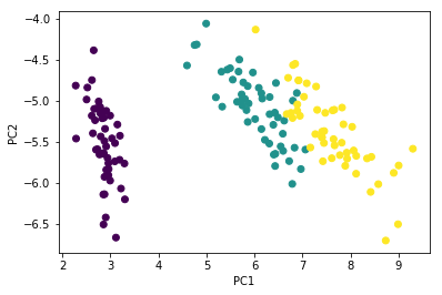
PCA is \(U \Sigma\)
In [15]:
Y = U[:, :2] @ np.diag(s[:2])
In [16]:
plt.scatter(Y[:, 0], Y[:, 1],
            c=iris['Species'].astype('category').cat.codes)
plt.xlabel('PC1')
plt.ylabel('PC2')
pass

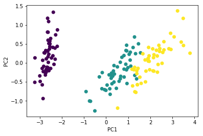
PCA is also \(XV\)
In [17]:
Z = X @ Vt.T[:, :2]
In [18]:
plt.scatter(Z[:, 0], Z[:, 1],
            c=iris['Species'].astype('category').cat.codes)
plt.xlabel('PC1')
plt.ylabel('PC2')
pass
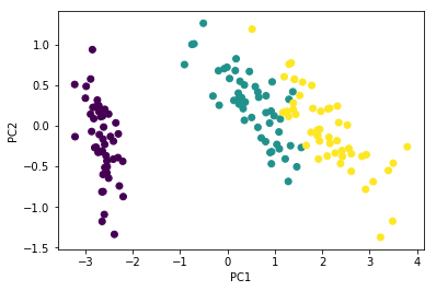
Check with PCA routine. It should be the same (eigenvectors may flip)
In [19]:
from sklearn.decomposition import PCA
In [20]:
pca = PCA(n_components=2)
In [21]:
Y1 = pca.fit_transform(Xc)
In [22]:
plt.scatter(Y1[:, 0], Y1[:, 1],
            c=iris['Species'].astype('category').cat.codes)
plt.xlabel('PC1')
plt.ylabel('PC2')
pass
Flip directions for the second eigenvector
In [60]:
plt.scatter(Y1[:, 0], -Y1[:, 1],
            c=iris['Species'].astype('category').cat.codes)
plt.xlabel('PC1')
plt.ylabel('PC2')
pass
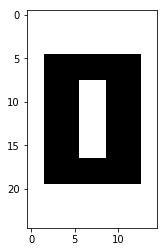
Data compression (Low rank approximations)
In [23]:
X = np.ones((25, 15))
X[5:-5, 2:-2] = 0
X[8:-8, 6:-6] = 1
In [24]:
plt.imshow(X, cmap='gray')
pass

In [25]:
U, s, Vt = la.svd(X, full_matrices=False)
Note that tehre are only 3 types of columns, and so 3 singular values suffice to capture all the information.
In [26]:
np.cumsum(s)/s.sum()
Out[26]:
array([ 0.6,  0.9,  1.0,  1.0,  1.0,  1.0,  1.0,  1.0,  1.0,  1.0,  1.0,
        1.0,  1.0,  1.0,  1.0])
In [27]:
X1 = U[:, :3] @ np.diag(s[:3]) @ Vt[:3, :]
In [28]:
plt.imshow(X, cmap='gray')
pass
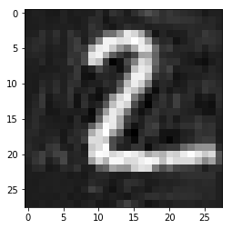
Using MNIST example
In [29]:
mnist = pd.read_csv('https://pjreddie.com/media/files/mnist_test.csv')
In [30]:
mnist.shape
Out[30]:
(9999, 785)
In [31]:
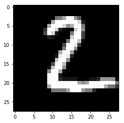
img = mnist.iloc[0, :-1].values.reshape((28,28))
In [32]:
plt.imshow(img, cmap='gray')
pass
In [33]:
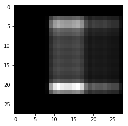
U, s, Vt = la.svd(img, full_matrices=False)
In [34]:
img1 = U[:, :1] @ np.diag(s[:1]) @ Vt[:1, :]
In [35]:
plt.imshow(img1, cmap='gray')
pass
In [36]:
np.cumsum(s)/s.sum()
Out[36]:
array([ 0.3,  0.5,  0.6,  0.7,  0.8,  0.9,  0.9,  0.9,  0.9,  0.9,  1.0,
        1.0,  1.0,  1.0,  1.0,  1.0,  1.0,  1.0,  1.0,  1.0,  1.0,  1.0,
        1.0,  1.0,  1.0,  1.0,  1.0,  1.0])
In [37]:
k = 6
imgk = U[:, :k] @ np.diag(s[:k]) @ Vt[:k, :]
In [38]:
plt.imshow(imgk, cmap='gray')
pass
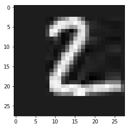
We get slightly more than 50% compression with \(k=6\). Note that there are better methods for image compression.
In [39]:
sizes = (U[:, :k].size, s[:k].size, Vt[:k, :].size)
In [40]:
sizes
Out[40]:
(168, 6, 168)
In [41]:
img.size
Out[41]:
784
In [42]:
sum(sizes)
Out[42]:
342
Denoising
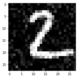
SVD by itself can do some denoising, but effective use requires more sophisticated algorithms such as k-SVD
In [43]:
img_noise = np.clip(img + np.random.normal(0, 30, img.shape), 0, 255)
In [44]:
plt.imshow(img_noise, cmap='gray')
pass
In [45]:
U, s, Vt = la.svd(img_noise, full_matrices=False)
In [46]:
np.cumsum(s)/s.sum()
Out[46]:
array([ 0.3,  0.4,  0.5,  0.6,  0.7,  0.7,  0.7,  0.8,  0.8,  0.8,  0.8,
        0.9,  0.9,  0.9,  0.9,  0.9,  0.9,  0.9,  1.0,  1.0,  1.0,  1.0,
        1.0,  1.0,  1.0,  1.0,  1.0,  1.0])
In [47]:
k = 6
imgk_noise = U[:, :k] @ np.diag(s[:k]) @ Vt[:k, :]
In [48]:
plt.imshow(imgk_noise, cmap='gray')
pass
Recommender system
Based on toy example from this blog post
In [49]:
from collections import OrderedDict
We have a database of movies and user ratings, but since most users watch and rate only a small subset of all possible movies, there is a lot of missing data. Our job is to predict what other movies a user might like, based on the movies that the user has rated.
Recall that SVD gives the optimal (in terms of Frobenius norm) low rank reconstruction for a matrix. This is true even for sparse matrices, and we make use of this to make predictions about user movie preferences.
Note: Real world recommender systems based on SVD calculate an approximate SVD using iterative methods for computational efficiency, but the idea is the same - we assume that the data can be modeled by \(k\) latent factors, then reconstruct the rank-\(k\) matrix. You’d also normalize the data in a real-use case.
In [50]:
ratings = pd.SparseDataFrame.from_dict(OrderedDict(
    A = [2,None,2,4,5,None],
    B = [5,None,4,None,None,1],
    C = [None,None,5,None,2,None],
    D = [None,1,None,5,None,4],
    E = [None,None,4,None,None,2,],
    F = [4,5,None,1,None,None]), orient='index'
)
ratings.columns = ['The Avengers', 'Sherlock', 'Transformers', 'Matrix', 'Titanic', 'Me Before You']
In [51]:
ratings
Out[51]:
| The Avengers | Sherlock | Transformers | Matrix | Titanic | Me Before You | |
|---|---|---|---|---|---|---|
| A | 2.0 | NaN | 2.0 | 4.0 | 5.0 | NaN |
| B | 5.0 | NaN | 4.0 | NaN | NaN | 1.0 |
| C | NaN | NaN | 5.0 | NaN | 2.0 | NaN |
| D | NaN | 1.0 | NaN | 5.0 | NaN | 4.0 |
| E | NaN | NaN | 4.0 | NaN | NaN | 2.0 |
| F | 4.0 | 5.0 | NaN | 1.0 | NaN | NaN |
We need to deal with the sparsity.
In [52]:
from scipy.sparse.linalg import svds
In [53]:
X = ratings.to_coo()
In [54]:
print(X)
  (0, 0)        2.0
  (1, 0)        5.0
  (5, 0)        4.0
  (3, 1)        1.0
  (5, 1)        5.0
  (0, 2)        2.0
  (1, 2)        4.0
  (2, 2)        5.0
  (4, 2)        4.0
  (0, 3)        4.0
  (3, 3)        5.0
  (5, 3)        1.0
  (0, 4)        5.0
  (2, 4)        2.0
  (1, 5)        1.0
  (3, 5)        4.0
  (4, 5)        2.0
In [55]:
U, s, Vt = svds(X, k=min(ratings.shape)-1)
In [56]:
s
Out[56]:
array([ 3.0, 4.9, 6.4, 6.9, 10.1])
svds gives singular values in ascending order, so we need to perform a permutation to get it in the fmiliar form.
In [57]:
perm = np.arange(len(s))[::-1]
U = U[:, perm]
s = s[perm]
Vt = Vt[perm, :]
In [58]:
k = 3
Y = U[:, :k] @ np.diag(s[:k]) @ Vt[:k, :]
Y
Out[58]:
array([[ 1.4,  0.4,  2.9,  4.0,  2.7,  2.1],
       [ 4.0,  1.5,  4.2, -0.2,  1.0,  0.2],
       [ 0.9, -1.1,  4.6,  0.0,  1.8,  0.4],
       [ 0.3,  1.0, -0.6,  5.0,  1.9,  2.3],
       [ 0.7, -0.7,  3.3,  0.2,  1.4,  0.4],
       [ 4.7,  4.0, -0.2,  1.1, -0.5,  0.4]])
In [59]:
user = 'E'
pd.DataFrame(OrderedDict(
    Observed = ratings.loc[user].to_dense(),
    Predicted = Y[ratings.index.tolist().index(user)]))
Out[59]:
| Observed | Predicted | |
|---|---|---|
| The Avengers | NaN | 0.749016 |
| Sherlock | NaN | -0.688250 |
| Transformers | 4.0 | 3.292351 |
| Matrix | NaN | 0.243724 |
| Titanic | NaN | 1.360181 |
| Me Before You | 2.0 | 0.379015 |