Time Series Analysis 1
In the first lecture, we are mainly concerned with how to manipulate and smooth time series data.
In [1]:
%matplotlib inline
import matplotlib.pyplot as plt
In [2]:
import os
import time
In [3]:
import numpy as np
import pandas as pd
In [4]:
import gmaps
import gmaps.datasets
Dates and times
Timestamps
In [5]:
now = pd.to_datetime('now')
In [6]:
now
Out[6]:
Timestamp('2018-11-04 17:15:19.437536')
In [7]:
now.year, now.month, now.week, now.day, now.hour, now.minute, now.second, now.microsecond
Out[7]:
(2018, 11, 44, 4, 17, 15, 19, 437536)
In [8]:
now.month_name(), now.day_name()
Out[8]:
('November', 'Sunday')
Formatting timestamps
See format codes
In [9]:
now.strftime('%I:%m%p %d-%b-%Y')
Out[9]:
'05:11PM 04-Nov-2018'
Parsing time strings
pandas can handle standard formats
In [10]:
ts = pd.to_datetime('6-Dec-2018 4:45 PM')
In [11]:
ts
Out[11]:
Timestamp('2018-12-06 16:45:00')
For unusual formats, use strptime
In [12]:
ts = pd.datetime.strptime('10:11PM 02-Nov-2018', '%I:%m%p %d-%b-%Y')
In [13]:
ts
Out[13]:
datetime.datetime(2018, 11, 2, 22, 0)
Intervals
In [14]:
then = pd.to_datetime('now')
time.sleep(5)
now = pd.to_datetime('now')
In [15]:
now - then
Out[15]:
Timedelta('0 days 00:00:05.004077')
Date ranges
A date range is just a collection of time stamps.
In [16]:
dates = pd.date_range(then, now, freq='s')
In [17]:
dates
Out[17]:
DatetimeIndex(['2018-11-04 17:15:19.500621', '2018-11-04 17:15:20.500621',
               '2018-11-04 17:15:21.500621', '2018-11-04 17:15:22.500621',
               '2018-11-04 17:15:23.500621', '2018-11-04 17:15:24.500621'],
              dtype='datetime64[ns]', freq='S')
In [18]:
(then - pd.to_timedelta('1.5s')) in dates
Out[18]:
False
Periods
Periods are intervals, not a collection of timestamps.
In [19]:
span = dates.to_period()
In [20]:
span
Out[20]:
PeriodIndex(['2018-11-04 17:15:19', '2018-11-04 17:15:20',
             '2018-11-04 17:15:21', '2018-11-04 17:15:22',
             '2018-11-04 17:15:23', '2018-11-04 17:15:24'],
            dtype='period[S]', freq='S')
In [21]:
(then + pd.to_timedelta('1.5s')) in span
Out[21]:
True
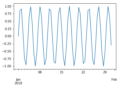
Lag and lead with shift
We will use a periodic time series as an example. Periodicity is important because many biological phenomena are linked to natural periods (seasons, diurnal, menstrual cycle) or are intrinsically periodic (e.g. EEG, EKG measurements).
In [22]:
index = pd.date_range('1-1-2018', '31-1-2018', freq='12h')
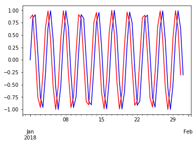
You can shift by periods or by frequency. Shifting by frequency maintains boundary data.
In [23]:
wave = pd.Series(np.sin(np.arange(len(index))), index=index)
In [24]:
wave.shift(periods=1).head(3)
Out[24]:
2018-01-01 00:00:00         NaN
2018-01-01 12:00:00    0.000000
2018-01-02 00:00:00    0.841471
Freq: 12H, dtype: float64
In [25]:
wave.shift(periods=1).tail(3)
Out[25]:
2018-01-30 00:00:00    0.436165
2018-01-30 12:00:00    0.992873
2018-01-31 00:00:00    0.636738
Freq: 12H, dtype: float64
In [26]:
wave.shift(freq=1).head(3)
Out[26]:
2018-01-01 12:00:00    0.000000
2018-01-02 00:00:00    0.841471
2018-01-02 12:00:00    0.909297
Freq: 12H, dtype: float64
In [27]:
wave.shift(freq=1).tail(3)
Out[27]:
2018-01-30 12:00:00    0.992873
2018-01-31 00:00:00    0.636738
2018-01-31 12:00:00   -0.304811
Freq: 12H, dtype: float64
In [28]:
wave.plot()
pass
In [29]:
wave.plot(c='blue')
wave.shift(-1).plot(c='red')
pass
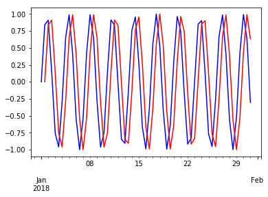
In [30]:
wave.plot(c='blue')
wave.shift(1).plot(c='red')
pass
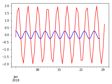
In [31]:
(wave - wave.shift(-6)).plot(c='blue')
(wave - wave.shift(-3)).plot(c='red')
pass
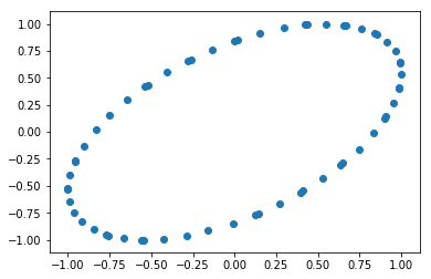
Embedding the time series with its lagged version reveals its periodic nature.
In [32]:
plt.scatter(wave, wave.shift(-1))
pass
Find percent change from previous period
In [33]:
wave.pct_change().head()
Out[33]:
2018-01-01 00:00:00         NaN
2018-01-01 12:00:00         inf
2018-01-02 00:00:00    0.080605
2018-01-02 12:00:00   -0.844803
2018-01-03 00:00:00   -6.362829
Freq: 12H, dtype: float64
pct_change is just a convenience wrapper around the use of shift
In [34]:
((wave - wave.shift(-1, freq='12h'))/wave).head()
Out[34]:
2017-12-31 12:00:00         NaN
2018-01-01 00:00:00        -inf
2018-01-01 12:00:00   -0.080605
2018-01-02 00:00:00    0.844803
2018-01-02 12:00:00    6.362829
Freq: 12H, dtype: float64
Resampling and window functions
The resample and window method have the same syntax as groupby,
in that you can apply an aggregate function to the new intervals.
Resampling
Sometimes there is a need to generate new time intervals, for example, to regularize irregularly timed observations.
Down-sampling
In [35]:
index = pd.date_range(pd.to_datetime('1-1-2018'), periods=365, freq='d')
In [36]:
series = pd.Series(np.arange(len(index)), index=index)
In [37]:
series.head()
Out[37]:
2018-01-01    0
2018-01-02    1
2018-01-03    2
2018-01-04    3
2018-01-05    4
Freq: D, dtype: int64
In [38]:
sereis_weekly_average = series.resample('w').mean()
sereis_weekly_average.head()
Out[38]:
2018-01-07     3
2018-01-14    10
2018-01-21    17
2018-01-28    24
2018-02-04    31
Freq: W-SUN, dtype: int64
In [39]:
sereis_monthly_sum = series.resample('m').sum()
sereis_monthly_sum.head()
Out[39]:
2018-01-31     465
2018-02-28    1246
2018-03-31    2294
2018-04-30    3135
2018-05-31    4185
Freq: M, dtype: int64
In [40]:
sereis_10day_median = series.resample('10d').median()
sereis_10day_median.head()
Out[40]:
2018-01-01     4.5
2018-01-11    14.5
2018-01-21    24.5
2018-01-31    34.5
2018-02-10    44.5
dtype: float64
Up-sampling
For up-sampling, we need to figure out what we want to do with the missing values. The usual choices are forward fill, backward fill, or interpolation using one of many built-in methods.
In [41]:
upsampled = series.resample('12h')
In [42]:
upsampled.asfreq()[:5]
Out[42]:
2018-01-01 00:00:00    0.0
2018-01-01 12:00:00    NaN
2018-01-02 00:00:00    1.0
2018-01-02 12:00:00    NaN
2018-01-03 00:00:00    2.0
Freq: 12H, dtype: float64
In [43]:
upsampled.ffill().head()
Out[43]:
2018-01-01 00:00:00    0
2018-01-01 12:00:00    0
2018-01-02 00:00:00    1
2018-01-02 12:00:00    1
2018-01-03 00:00:00    2
Freq: 12H, dtype: int64
In [44]:
upsampled.bfill().head()
Out[44]:
2018-01-01 00:00:00    0
2018-01-01 12:00:00    1
2018-01-02 00:00:00    1
2018-01-02 12:00:00    2
2018-01-03 00:00:00    2
Freq: 12H, dtype: int64
In [45]:
upsampled.interpolate('linear').head()
Out[45]:
2018-01-01 00:00:00    0.0
2018-01-01 12:00:00    0.5
2018-01-02 00:00:00    1.0
2018-01-02 12:00:00    1.5
2018-01-03 00:00:00    2.0
Freq: 12H, dtype: float64
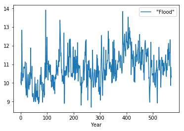
Window functions
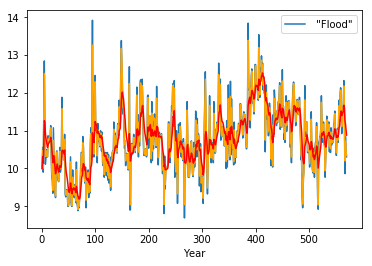
Window functions are typically used to smooth time series data. There are 3 variants - rolling, expanding and exponentially weighted. We use the Nile flooding data for these examples.
In [46]:
df = pd.read_csv('data/nile.csv', index_col=0)
In [47]:
df.head()
Out[47]:
| "Flood" | |
|---|---|
| Year | |
| 1 | 9.9974 |
| 2 | 10.5556 |
| 3 | 9.9014 |
| 4 | 11.4800 |
| 5 | 12.8460 |
In [48]:
df.plot()
pass
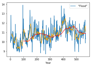
Rolling windows generate windows of a specified width
In [49]:
ts = pd.DataFrame(dict(ts=np.arange(5)))
ts['rolling'] = ts.rolling(window=3).sum()
ts
Out[49]:
| ts | rolling | |
|---|---|---|
| 0 | 0 | NaN |
| 1 | 1 | NaN |
| 2 | 2 | 3.0 |
| 3 | 3 | 6.0 |
| 4 | 4 | 9.0 |
In [50]:
rolling10 = df.rolling(window=10)
rolling100 = df.rolling(window=100)
In [51]:
df.plot()
plt.plot(rolling10.mean(), c='orange')
plt.plot(rolling100.mean(), c='red')
pass
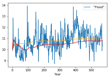
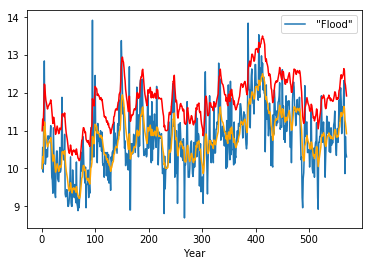
Expanding windows grow as the time series progresses
In [52]:
ts['expanding'] =  ts.ts.expanding().sum()
ts
Out[52]:
| ts | rolling | expanding | |
|---|---|---|---|
| 0 | 0 | NaN | 0.0 |
| 1 | 1 | NaN | 1.0 |
| 2 | 2 | 3.0 | 3.0 |
| 3 | 3 | 6.0 | 6.0 |
| 4 | 4 | 9.0 | 10.0 |
In [53]:
df.plot()
plt.plot(df.expanding(center=True).mean(), c='orange')
plt.plot(df.expanding().mean(), c='red')
pass
Exponentially weighted windows place more weight on center of mass
In [54]:
n = 10
xs = np.arange(n, dtype='float')[::-1]
xs
Out[54]:
array([9., 8., 7., 6., 5., 4., 3., 2., 1., 0.])
Exponentially weighted windows without adjustment.
In [55]:
pd.Series(xs).ewm(alpha=0.8, adjust=False).mean()
Out[55]:
0    9.000000
1    8.200000
2    7.240000
3    6.248000
4    5.249600
5    4.249920
6    3.249984
7    2.249997
8    1.249999
9    0.250000
dtype: float64
Re-implementation for insight.
In [56]:
α = 0.8
ys = np.zeros_like(xs)
ys[0] = xs[0]
for i in range(1, len(xs)):
    ys[i] = (1-α)*ys[i-1] + α*xs[i]
ys
Out[56]:
array([9.        , 8.2       , 7.24      , 6.248     , 5.2496    ,
       4.24992   , 3.249984  , 2.2499968 , 1.24999936, 0.24999987])
Exponentially weighted windows with adjustment (default)
In [57]:
pd.Series(xs).ewm(alpha=0.8, adjust=True).mean()
Out[57]:
0    9.000000
1    8.166667
2    7.225806
3    6.243590
4    5.248399
5    4.249616
6    3.249910
7    2.249980
8    1.249995
9    0.249999
dtype: float64
Re-implementation for insight.
In [58]:
α = 0.8
ys = np.zeros_like(xs)
ys[0] = xs[0]
for i in range(1, len(xs)):
    ws = np.array([(1-α)**(i-t) for t in range(i+1)])
    ys[i] = (ws * xs[:len(ws)]).sum()/ws.sum()
ys
Out[58]:
array([9.        , 8.16666667, 7.22580645, 6.24358974, 5.24839949,
       4.24961598, 3.2499104 , 2.24997952, 1.24999539, 0.24999898])
In [59]:
df.plot()
plt.plot(df.ewm(alpha=0.8).mean(), c='orange')
plt.plot(df.ewm(alpha=0.2).mean(), c='red')
pass
Alternatives to \(\alpha\)
Using span
Using halflife
Using com
In [60]:
df.plot()
plt.plot(df.ewm(span=10).mean(), c='orange')
plt.plot(1+ df.ewm(alpha=2/11).mean(), c='red') # offfset for visibility
pass
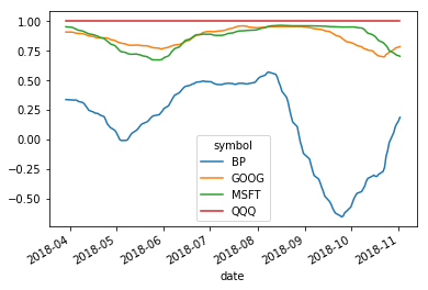
Correlation between time series
Suppose we had a reference time series. It is often of interest to know how any particular time series is correlated with the reference. Often the reference might be a population average, and we want to see where a particular time series deviates in behavior.
In [61]:
import pandas_datareader.data as web
We will look at the correlation of some stocks.
QQQ tracks Nasdaq
MSFT is Microsoft
GOOG is Gogole
BP is British Petroleum
We expect that the technology stocks should be correlated with Nasdaq, but maybe not BP.
In [62]:
df = web.DataReader(['QQQ', 'MSFT','GOOG', 'BP'], 'robinhood')
In [63]:
df = df[['close_price']]
In [64]:
df = df.unstack(level=0)
In [65]:
df.columns = df.columns.get_level_values(1)
In [66]:
df.index.name = 'date'
In [67]:
df.index = pd.to_datetime(df.index)
In [68]:
df.head()
Out[68]:
| symbol | BP | GOOG | MSFT | QQQ |
|---|---|---|---|---|
| date | ||||
| 2017-11-03 | 38.839900 | 1032.480000 | 82.643000 | 152.102400 |
| 2017-11-06 | 39.653900 | 1025.900000 | 82.967200 | 152.618500 |
| 2017-11-07 | 39.720900 | 1033.330000 | 82.770700 | 152.707800 |
| 2017-11-08 | 39.644300 | 1039.850000 | 83.055600 | 153.323100 |
| 2017-11-09 | 39.582200 | 1031.260000 | 82.593900 | 152.519200 |
In [69]:
df.rolling(100).corr(df.QQQ).plot()
pass
Visualizing space and time data
Being able to visualize events in space and time can be impressive. With Python, often you need a trivial amount of code to produce an impressive visualization.
For example, lets generate a heatmap of crimes in Sacramento in 2006, and highlight the crimes committed 10 seconds before midnight.
See the gmaps package for more information.
In [70]:
sacramento_crime = pd.read_csv('data/SacramentocrimeJanuary2006.csv', index_col=0)
In [71]:
sacramento_crime.index = pd.to_datetime(sacramento_crime.index)
In [72]:
sacramento_crime.head()
Out[72]:
| address | district | beat | grid | crimedescr | ucr_ncic_code | latitude | longitude | |
|---|---|---|---|---|---|---|---|---|
| cdatetime | ||||||||
| 2006-01-01 | 3108 OCCIDENTAL DR | 3 | 3C | 1115 | 10851(A)VC TAKE VEH W/O OWNER | 2404 | 38.550420 | -121.391416 |
| 2006-01-01 | 2082 EXPEDITION WAY | 5 | 5A | 1512 | 459 PC BURGLARY RESIDENCE | 2204 | 38.473501 | -121.490186 |
| 2006-01-01 | 4 PALEN CT | 2 | 2A | 212 | 10851(A)VC TAKE VEH W/O OWNER | 2404 | 38.657846 | -121.462101 |
| 2006-01-01 | 22 BECKFORD CT | 6 | 6C | 1443 | 476 PC PASS FICTICIOUS CHECK | 2501 | 38.506774 | -121.426951 |
| 2006-01-01 | 3421 AUBURN BLVD | 2 | 2A | 508 | 459 PC BURGLARY-UNSPECIFIED | 2299 | 38.637448 | -121.384613 |
In [73]:
gmaps.configure(api_key=os.environ["GOOGLE_API_KEY"])
In [74]:
locations = sacramento_crime[['latitude', 'longitude']]
In [75]:
late_locations = sacramento_crime.between_time('23:59', '23:59:59')[['latitude', 'longitude']]
In [76]:
fig = gmaps.figure()
fig.add_layer(gmaps.heatmap_layer(locations))
markers = gmaps.marker_layer(late_locations)
fig.add_layer(markers)
fig