Statistics review 10: Further nonparametric methods
R code accompanying
paper
Key learning points
- Nonparametric methods for testing differences between more than two
groups or treatments
suppressPackageStartupMessages(library(tidyverse))
options(repr.plot.width=4, repr.plot.height=3)
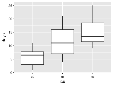
Kruskal–Wallis test
Nonparametric alternative to one-way analysis of variance.
Manual calculation
ct <- c(7,1,2,6,11,8)
m <- c(4,7,16,11,21)
ns <- c(20,25,13,9,14,11)
icu <- c(rep("ct", length(ct)), rep("m", length(m)), rep("ns", length(ns)))
days <- c(ct, m, ns)

df <- data.frame(icu=icu, days=days)
| icu | days |
|---|
| ct | 7 |
| ct | 1 |
| ct | 2 |
| ct | 6 |
| ct | 11 |
| ct | 8 |
ggplot(df, aes(x=icu, y=days)) + geom_boxplot()
df1 <- df %>% mutate(rank=rank(days))
head(df1)
| icu | days | rank |
|---|
| ct | 7 | 5.5 |
| ct | 1 | 1.0 |
| ct | 2 | 2.0 |
| ct | 6 | 4.0 |
| ct | 11 | 10.0 |
| ct | 8 | 7.0 |
df2 <- df1 %>% group_by(icu) %>% summarize(r = sum(rank), n=n())
df2
| icu | r | n |
|---|
| ct | 29.5 | 6 |
| m | 48.5 | 5 |
| ns | 75.0 | 6 |
N <- dim(df1)[1]

T <- (12/(N*(N+1)))*sum((df2$r^2/df2$n)) - 3*(N+1)
6.9
2
round(1 - pchisq(T, df), 4)
0.0317
Using built in function
kruskal.test(days ~ icu, data=df1)
    Kruskal-Wallis rank sum test

data:  days by icu
Kruskal-Wallis chi-squared = 6.9442, df = 2, p-value = 0.03105
Dunn test for multiple comparisons
suppressPackageStartupMessages(library(FSA))
dunnTest(df1$days, df1$icu)
Dunn (1964) Kruskal-Wallis multiple comparison
  p-values adjusted with the Holm method.
  Comparison          Z    P.unadj      P.adj
1     ct - m -1.5691321 0.11661717 0.23323435
2    ct - ns -2.6090676 0.00907893 0.02723679
3     m - ns -0.9185163 0.35834862 0.35834862
Ad-hoc comparisons with Wilcoxon
pairwise.wilcox.test(df1$days, df1$icu, p.adjust.method = "holm")
Warning message in wilcox.test.default(xi, xj, paired = paired, ...):
“cannot compute exact p-value with ties”Warning message in wilcox.test.default(xi, xj, paired = paired, ...):
“cannot compute exact p-value with ties”Warning message in wilcox.test.default(xi, xj, paired = paired, ...):
“cannot compute exact p-value with ties”
    Pairwise comparisons using Wilcoxon rank sum test

data:  df1$days and df1$icu

   ct    m
m  0.338 -
ns 0.031 0.464

P value adjustment method: holm
The Jonckheere–Terpstra test
For comparisons where the treatment group is ordinal.
We re-use the same data set, assuming that the ICU ordering is ct, m,
ns.
Using a package
| icu | days | rank |
|---|
| ct | 7 | 5.5 |
| ct | 1 | 1.0 |
| ct | 2 | 2.0 |
| ct | 6 | 4.0 |
| ct | 11 | 10.0 |
| ct | 8 | 7.0 |
df1$icu <- factor(df1$icu, levels=c("ct", "m","ns"))
'data.frame':       17 obs. of  3 variables:
 $ icu : Factor w/ 3 levels "ct","m","ns": 1 1 1 1 1 1 2 2 2 2 ...
 $ days: num  7 1 2 6 11 8 4 7 16 11 ...
 $ rank: num  5.5 1 2 4 10 7 3 5.5 14 10 ...
jonckheere.test(df1$days, as.numeric(df1$icu), nperm=10000)
    Jonckheere-Terpstra test

data:
JT = 77, p-value = 0.0102
alternative hypothesis: two.sided
- 7
- 1
- 2
- 6
- 11
- 8
- 4
- 7
- 16
- 11
- 21
- 20
- 25
- 13
- 9
- 14
- 11
- 1
- 1
- 1
- 1
- 1
- 1
- 2
- 2
- 2
- 2
- 2
- 3
- 3
- 3
- 3
- 3
- 3
The Friedman Test
Extension of the sign test for matched pairs and is used when the data
arise from more than two related samples. The Friedman test is the
non-parametric alternative to the one-way ANOVA with repeated measures.
Used as a two-way ANOVA with a completely balanced design.
A <- c(6,9,10,14,11)
B <- c(9,16,14,14,16)
C <- c(10,16,22,40,17)
D <- c(16,32,67,19,60)

df3 <- data.frame(Patient = 1:5, A=A, B=B, C=C, D=D)
df3.rank <- t(apply(df3[,2:5], 1, rank))
df3.rank <- data.frame(df3.rank)
df3.rank
| A | B | C | D |
|---|
| 1.0 | 2.0 | 3.0 | 4 |
| 1.0 | 2.5 | 2.5 | 4 |
| 1.0 | 2.0 | 3.0 | 4 |
| 1.5 | 1.5 | 4.0 | 3 |
| 1.0 | 2.0 | 3.0 | 4 |
df4 <- df3.rank %>% summarise_each("sum")
df4
k <- dim(df3.rank)[2]
b <- dim(df3.rank)[1]

T <- (12/(b*k*(k+1)))*sum(df4^2) - 3*b*(k+1)
12.78
round(1 - pchisq(T, k-1), 4)
0.0051
| Patient | A | B | C | D |
|---|
| 1 | 6 | 9 | 10 | 16 |
| 2 | 9 | 16 | 16 | 32 |
| 3 | 10 | 14 | 22 | 67 |
| 4 | 14 | 14 | 40 | 19 |
| 5 | 11 | 16 | 17 | 60 |
df5 <- df3 %>% gather(treatment, score, A:D)
head(df5)
| Patient | treatment | score |
|---|
| 1 | A | 6 |
| 2 | A | 9 |
| 3 | A | 10 |
| 4 | A | 14 |
| 5 | A | 11 |
| 1 | B | 9 |
'data.frame':       20 obs. of  3 variables:
 $ Patient  : int  1 2 3 4 5 1 2 3 4 5 ...
 $ treatment: chr  "A" "A" "A" "A" ...
 $ score    : num  6 9 10 14 11 9 16 14 14 16 ...
friedman.test(score ~ treatment | Patient, data=df5)
    Friedman rank sum test

data:  score and treatment and Patient
Friedman chi-squared = 13.312, df = 3, p-value = 0.004007
friedman.test(df5$score, df5$treatment, df5$Patient)
    Friedman rank sum test

data:  df5$score, df5$treatment and df5$Patient
Friedman chi-squared = 13.312, df = 3, p-value = 0.004007
| weight | feed |
|---|
| 179 | horsebean |
| 160 | horsebean |
| 136 | horsebean |
| 227 | horsebean |
| 217 | horsebean |
| 168 | horsebean |
Exercise
1. Practice using the non-parametric tests on the chickwts data
set.