Numerical Evaluation of Integrals

Integration problems are common in statistics whenever we are dealing with continuous distributions. For example the expectation of a function is an integration problem

\begin{align} E[f(x)] = \int{f(x) \, p(x) \, dx} \end{align}

In Bayesian statistics, we need to solve the integration problem for the marginal likelihood or evidence

\[p(X \mid \alpha) = \int{p(X \mid \theta) \, p(\theta \mid \alpha) d\theta}\]

where \(\alpha\) is a hyperparameter and \(p(X \mid \alpha)\) appears in the denominator of Bayes theorem

\[p(\theta \mid X) = \frac{p(X \mid \theta) \, p(\theta \mid \alpha)}{p(X \mid \alpha)}\]

Knowing the marginal likelihood will allow evaluation of the posterior in some cases.

In general, there is no closed form solution to these integrals, and we have to approximate them numerically. The first step is to check if there is some reparameterization that will simplify the problem. Then, the general approaches to solving integration problems are

1. Numerical quadrature
2. Importance sampling, adaptive importance sampling and variance reduction techniques (Monte Carlo swindles)
3. Markov Chain Monte Carlo
4. Asymptotic approximations (Laplace method and its modern version in variational inference)

This lecture will review the concepts for quadrature and Monte Carlo integration.

Quadrature

You may recall from Calculus that integrals can be numerically evaluated using quadrature methods such as Trapezoid and Simpson’s‘s rules. This is easy to do in Python, but has the drawback of the complexity growing as \(O(n^d)\) where \(d\) is the dimensionality of the data, and hence infeasible once \(d\) grows beyond a modest number. In low dimensions, however, quadrature will give a slightly better estimate than Monte Carlo integration for a given number of points used in estimation (partitions in quadrature, samples in Monte Carlo).

Integrating functions

The scipy package contains a function to perform quadrature, called quad.

In [1]:

from scipy.integrate import quad
import numpy as np
import matplotlib.pyplot as plt
%matplotlib inline

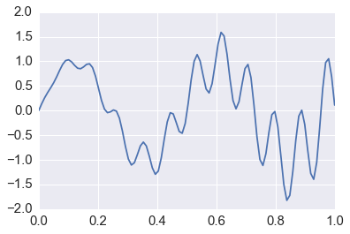
We will demonstrate quadrature on the function \(f(x) = x\cos{71x} + \sin{13x}\), which is plotted below.

In [2]:

def f(x):
    return x * np.cos(71*x) + np.sin(13*x)

In [3]:

x = np.linspace(0, 1, 100)
plt.plot(x, f(x))
pass

Exact solution

For reference we will get an ‘exact’ solution using sympy to evaluate the expression to six significant digits.

In [4]:

from sympy import sin, cos, symbols, integrate

x = symbols('x')
integrate(x * cos(71*x) + sin(13*x), (x, 0,1)).evalf(6)

Out[4]:

0.0202549

Using quadrature

We will now calculate the value using quadrature. We see the the values are equal

In [5]:

y, err = quad(f, 0, 1.0)
y

Out[5]:

0.02025493910239419

Multiple integration

Following the scipy.integrate documentation, we integrate

\[I=\int_{y=0}^{1/2}\int_{x=0}^{1-2y} x y \, dx\, dy\]

In [6]:

x, y = symbols('x y')
integrate(x*y, (x, 0, 1-2*y), (y, 0, 0.5))

Out[6]:

0.0104166666666667

In [7]:

from scipy.integrate import nquad

def f(x, y):
    return x*y

def bounds_y():
    return [0, 0.5]

def bounds_x(y):
    return [0, 1-2*y]

y, err = nquad(f, [bounds_x, bounds_y])
y

Out[7]:

0.010416666666666668

Monte Carlo integration

The basic idea of Monte Carlo integration is very simple and only requires elementary statistics. Suppose we want to find the value of

\[I = \int_a^b f(x) dx\]

in some region with volume \(V\). Monte Carlo integration estimates this integral by estimating the fraction of random points that fall below \(f(x)\) multiplied by \(V\).

In a statistical context, we use Monte Carlo integration to estimate the expectation

\[E[g(X)] = \int_X g(x) p(x) dx\]

with

\[\bar{g_n} = \frac{1}{n} \sum_{i=1}^n g(x_i)\]

where \(x_i \sim p\) is a draw from the density \(p\).

We can estimate the Monte Carlo variance of the approximation as

\[v_n = \frac{1}{n^2} \sum_{o=1}^n (g(x_i) - \bar{g_n})^2)\]

Also, from the Central Limit Theorem,

\[\frac{\bar{g_n} - E[g(X)]}{\sqrt{v_n}} \sim \mathcal{N}(0, 1)\]

The convergence of Monte Carlo integration is \(\mathcal{0}(n^{1/2})\) and independent of the dimensionality. Hence Monte Carlo integration generally beats numerical integration for moderate- and high-dimensional integration since numerical integration (quadrature) converges as \(\mathcal{0}(n^{d})\). Even for low dimensional problems, Monte Carlo integration may have an advantage when the volume to be integrated is concentrated in a very small region and we can use information from the distribution to draw samples more often in the region of importance.

An elementary, readable description of Monte Carlo integration and variance reduction techniques can be found here.

Intuition behind Monte Carlo integration

We want to find some integral

\[I = \int{f(x)} \, dx\]

Consider the expectation of a function \(g(x)\) with respect to some distribution \(p(x)\). By defiitinon, we have

\[E[g(x)] = \int{g(x) \, p(x) \, dx}\]

If we choose \(g(x) = f(x)/p(x)\), then we have

\begin{align} E[g(x)] &= \int{\frac{f(x)}{p(x)} \, p(x) \, dx} \\ &= \int{f(x) dx} \\ &= I \end{align}

By the law of large numbers, the average converges on the expectation, so we have

\[I \approx \bar{g_n} = \frac{1}{n} \sum_{i=1}^n g(x_i)\]

If \(f(x)\) is a proper integral (i.e. bounded), and \(p(x)\) is the uniform distribution, then \(g(x) = f(x)\) and this is known as ordinary Monte Carlo. If \(f(x)\) is imporper, then we need to use another distribtuion with the same support as \(f(x)\).

Intuition for error rate

We will just work this out for a proper integral \(f(x)\) defined in the unit cube and bounded by \(|f(x)| \le 1\). Draw a random uniform vector \(x\) in the unit cube. Then

\begin{align} E[f(x_i)] &= \int{f(x) p(x) dx} = I & \text{Definition of expectation} \\ \text{Var}[f(x_i)] &= \int{(f(x_i) - I )^2 p(x) \, dx} & \text{Definition of variance} \\ &= \int{f(x)^2 \, p(x) \, dx} - 2I \int f(x) \, p(x) \, dx + I^2 \int{p(x) \, dx} \\ &= \int{f(x)^2 \, p(x) \, dx} - I^2 & \text{because } \int p(x) \, dx = 1\\ & \le \int{f(x)^2 \, p(x) \, dx} & I^2 \geq 0 \\ & \le \int{p(x) \, dx} = 1 & |f(x)| \leq 1 \end{align}

Now consider summing over many such IID draws \(S_n = f(x_1) + f(x_2) + \cdots + f(x_n)\). We have

\begin{align} E[S_n] &= nI \\ \text{Var}[S_n] & \le n \end{align}

and as expected, we see that \(I \approx S_n/n\) (the average of \(f\) evaluated at the draws). From Chebyshev’s inequality,

\begin{align} P \left( \left| \frac{s_n}{n} - I \right| \ge \epsilon \right) &= P \left( \left| s_n - nI \right| \ge n \epsilon \right) \\ & \le \frac{\text{Var}[s_n]}{n^2 \epsilon^2} \\ & \le \frac{1}{n \epsilon^2} = \delta \end{align}

Suppose we want the estimate within 0.01 of the true value (\(I\)) with 99% confidence - i.e. set \(\epsilon = \delta = 0.01\). The above inequality tells us that we can achieve this with just \(n = 1/(\delta \epsilon^2) = 1,000,000\) samples, regardless of the data dimensionality.

Example

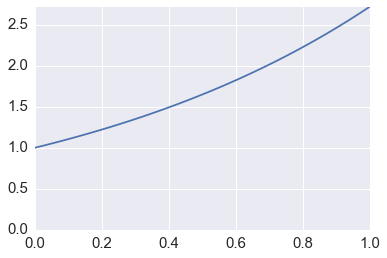
We want to estimate the following integral \(\int_0^1 e^x dx\). The minimum value of the function is 1 at \(x=0\) and \(e\) at \(x=1\).

In [8]:

x = np.linspace(0, 1, 100)
plt.plot(x, np.exp(x))
plt.xlim([0,1])
plt.ylim([0, np.e])
pass

Analytic solution

First we find the analytic solution using sympy.

In [9]:

from sympy import symbols, integrate, exp

x = symbols('x')
expr = integrate(exp(x), (x,0,1))
expr.evalf()

Out[9]:

1.71828182845905

Using quadrature

Then we estiamte using quadrature.

In [10]:

from scipy import integrate

y, err = integrate.quad(exp, 0, 1)
y

Out[10]:

1.7182818284590453

Monte Carlo integration

Now we use Monte Carlo integration with various \(n\).

In [11]:

for n in 10**np.array([1,2,3,4,5,6,7,8]):
    x = np.random.uniform(0, 1, n)
    sol = np.mean(np.exp(x))
    print('%10d %.6f' % (n, sol))

        10 1.869352
       100 1.780298
      1000 1.709496
     10000 1.717796
    100000 1.718669
   1000000 1.718052
  10000000 1.718253
 100000000 1.718267

Note that even with \(10^8\) samples, the Monte Carlo estimate is still less accurate than the answer obtained from quadrature.

Monitoring variance in Monte Carlo integration

We are often interested in knowing how many iterations it takes for Monte Carlo integration to “converge”. To do this, we would like some estimate of the variance, and it is useful to inspect such plots. One simple way to get confidence intervals for the plot of Monte Carlo estimate against number of iterations is simply to do many such simulations.

For the example, we will try to estimate the function (again)

\[f(x) = x \cos 7x + \sin 13x, \ \ 0 \le x \le 1\]

In [12]:

def f(x):
    return x * np.cos(71*x) + np.sin(13*x)

In [13]:

x = np.linspace(0, 1, 100)
plt.plot(x, f(x))
pass

Single MC integration estimate

In [14]:

n = 100
x = f(np.random.random(n))
y = 1.0/n * np.sum(x)
y

Out[14]:

0.11667355233523695

Using multiple independent sequences to monitor convergence

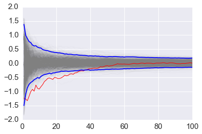
We vary the sample size from 1 to 100 and calculate the value of \(y = \sum{x}/n\) for 1000 replicates. We then plot the 2.5th and 97.5th percentile of the 1000 values of \(y\) to see how the variation in \(y\) changes with sample size. The blue lines indicate the 2.5th and 97.5th percentiles, and the red line a sample path.

In [15]:

n = 100
reps = 1000
# draw 1000 sets of 100 samples
x = f(np.random.random((n, reps)))
# compte running averages
y = 1/np.arange(1, n+1)[:, None] * np.cumsum(x, axis=0)
# get percentiles
upper, lower = np.percentile(y, [2.5, 97.5], axis=1)

In [16]:

# plot all sample lines with transperency in grey
plt.plot(np.arange(1, n+1), y, c='grey', alpha=0.02)
# plot the first column as a sample sequence in red
plt.plot(np.arange(1, n+1), y[:, 0], c='red', linewidth=1);
# plot the 2.5% and 97.5% bound lines in blue
plt.plot(np.arange(1, n+1), upper, 'b', np.arange(1, n+1), lower, 'b')
pass

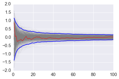
Using bootstrap to monitor convergence

If it is too expensive to do 1000 replicates, we can use a bootstrap instead. We will reuse the first set of 100 samples from the code above.

In [17]:

# sample with replacement from x[:,0]
# here we are resampling the 100 draws from our previous estimate (the bootstrap)
xb = np.random.choice(x[:,0], (n, reps), replace=True)
# compute the running average
yb = 1/np.arange(1, n+1)[:, None] * np.cumsum(xb, axis=0)
# get the percentiles
upper, lower = np.percentile(yb, [2.5, 97.5], axis=1)

In [18]:

# plot all samples in grey with transperancy
plt.plot(np.arange(1, n+1)[:, None], yb, c='grey', alpha=0.02)
# plot first running average in red
plt.plot(np.arange(1, n+1), yb[:, 0], c='red', linewidth=1)
# plot 2.5 and 97.5 bounds
plt.plot(np.arange(1, n+1), upper, 'b', np.arange(1, n+1), lower, 'b')
pass

Variance Reduction

With independent samples, the variance of the Monte Carlo estimate is

\begin{align} \text{Var}[\bar{g_n}] &= \text{Var} \left[ \frac{1}{N}\sum_{i=1}^{N} \frac{f(x_i)}{p(x_i)} \right] \\ &= \frac{1}{N^2} \sum_{i=1}^{N} \text{Var} \left[ \frac{f(x_i)}{p(x_i)} \right] \\ &= \frac{1}{N^2} \sum_{i=1}^{N} \text{Var}[Y_i] \\ &= \frac{1}{N} \text{Var}[Y_i] \end{align}

where \(Y_i = f(x_i)/p(x_i)\). The objective of Monte Carlo swindles is to make \(\text{Var}[\bar{g_n}]\) as small as possible for the same number of samples.

Change of variables

The Cauchy distribution is given by

\[f(x) = \frac{1}{\pi (1 + x^2)}, \ \ -\infty \lt x \lt \infty\]

Suppose we want to integrate the tail probability \(P(X > 3)\) using Monte Carlo. One way to do this is to draw many samples from a Cauchy distribution, and count how many of them are greater than 3, but this is extremely inefficient.

Only 10% of samples will be used

In [19]:

import scipy.stats as stats
# compute the true value
h_true = 1 - stats.cauchy().cdf(3)
h_true

Out[19]:

0.10241638234956674

In [20]:

# use 100 samples
n = 100
# draw samples from Cauchy
x = stats.cauchy().rvs(n)
# count number greater than 3
h_mc = 1.0/n * np.sum(x > 3)
# print estimate and error
h_mc, np.abs(h_mc - h_true)/h_true

Out[20]:

(0.10000000000000001, 0.023593709269276428)

A change of variables lets us use 100% of draws

We are trying to estimate the quantity

\int_3^\infty \frac{1}{\pi (1 + x^2)} dx

Using the substitution \(y = 3/x\) (and a little algebra), we get

\int_0^1 \frac{3}{\pi(9 + y^2)} dy

Hence, a much more efficient MC estimator is

\frac{1}{n} \sum_{i=1}^n \frac{3}{\pi(9 + y_i^2)}

where \(y_i \sim \mathcal{U}(0, 1)\).

In [21]:

y = stats.uniform().rvs(n)
h_cv = 1.0/n * np.sum(3.0/(np.pi * (9 + y**2)))
h_cv, np.abs(h_cv - h_true)/h_true

Out[21]:

(0.10197574007215225, 0.0043024589162941598)

Monte Carlo swindles

Apart from change of variables, there are several general techniques for variance reduction, sometimes known as Monte Carlo swindles since these methods improve the accuracy and convergence rate of Monte Carlo integration without increasing the number of Monte Carlo samples. Some Monte Carlo swindles are:

• importance sampling
• stratified sampling
• control variates
• antithetic variates
• conditioning swindles including Rao-Blackwellization and independent variance decomposition

Most of these techniques are not particularly computational in nature, so we will not cover them in the course. I expect you will learn them elsewhere. We will illustrate importance sampling and antithetic variables here as examples.

Antithetic variables

The idea behind antithetic variables is to choose two sets of random numbers that are negatively correlated, then take their average, so that the total variance of the estimator is smaller than it would be with two sets of IID random variables. This is because

\begin{align} \text{Var}((Y_1 + Y_2)/2) &= [\text{Var}(Y_1 + Y_2)]/4 \\ &= [\text{Var}(Y_1) + \text{Var}(Y_2) + \text{Cov}(Y_1, Y_2)]/4, \end{align}

so if the covariance between samples (\(Y_1\) and \(Y_2\) here) is negative, the variance of the average will be reduced. We will demonstrate this using our usual function on \([0,1]\).

In [22]:

def f(x):
    return x * np.cos(71*x) + np.sin(13*x)

In [23]:

from sympy import sin, cos, symbols, integrate

x = symbols('x')
sol = integrate(x * cos(71*x) + sin(13*x), (x, 0,1)).evalf(16)
sol

Out[23]:

0.02025493910239406

Vanilla Monte Carlo

In [24]:

n = 10000
u = np.random.random(n)
x = f(u)
y = 1.0/n * np.sum(x)
y, abs(y-sol)/sol

Out[24]:

(0.010552382438454633, 0.4790217642665052)

Antithetic variables use first half of u supplemented with 1-u

This works because the random draws are now negatively correlated, and hence the sum of the variances will be less than in the IID case, while the expectation is unchanged.

In [25]:

u = np.r_[u[:n//2], 1-u[:n//2]]
x = f(u)
y = 1.0/n * np.sum(x)
y, abs(y-sol)/sol

Out[25]:

(0.018758046700478734, 0.07390258713433484)

Importance sampling

Ordinary Monte Carlo sampling evaluates

\[E[g(X)] = \int_X g(x)\, p(x) \, dx\]

Using another distribution \(h(x)\) - the so-called “importance function”, we can rewrite the above expression as an expectation with respect to \(h\)

\[E_p[g(x)] \ = \ \int_X g(x) \frac{p(x)}{h(x)} h(x) dx \ = \ E_h\left[ \frac{g(X) p(X)}{h(X)} \right]\]

giving us the new estimator

\[\bar{g_n} = \frac{1}{n} \sum_{i=1}^n \frac{p(x_i)}{h(x_i)} g(x_i)\]

where \(x_i \sim g\) is a draw from the density \(h\). This is helpful if the distribution \(h\) has a similar shape as the function \(f(x)\) that we are integrating over, since we will draw more samples from places where the integrand makes a larger or more “important” contribution. This is very dependent on a good choice for the importance function \(h\). Two simple choices for \(h\) are scaling

\[h(x) = \frac{1}{a} p(x/a)\]

and translation

\[h(x) = p(x - a)\]

In these cases, the parameter \(a\) is typically chosen using some adaptive algorithm, giving rise to adaptive importance sampling. Alternatively, a different distribution can be chosen as shown in the example below. Selecting a poor importance function can actually increase the variance of the estimate.

Example

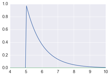
Suppose we want to estimate the tail probability of \(\mathcal{N}(0, 1)\) for \(P(X > 5)\). Regular MC integration using samples from \(\mathcal{N}(0, 1)\) is hopeless since nearly all samples will be rejected. However, we can use the exponential density truncated at 5 as the importance function and use importance sampling.

In [26]:

# domian for the plot
x = np.linspace(4, 10, 100)
# plot the exponential truncated at 5 in blue, our importance function
plt.plot(x, stats.expon(5).pdf(x))
# plot the tail of the normal distribution (in green)
plt.plot(x, stats.norm().pdf(x))
pass

Expected answer

We expect about 3 draws out of 10,000,000 from \(\mathcal{N}(0, 1)\) to have a value greater than 5. Hence simply sampling from \(\mathcal{N}(0, 1)\) is hopelessly inefficient for Monte Carlo integration.

In [27]:

%precision 10

Out[27]:

'%.10f'

In [28]:

h_true =1 - stats.norm().cdf(5)
h_true

Out[28]:

0.0000002867

Using direct Monte Carlo integration

In [29]:

# try 10000 samples
n = 10000
# draw from normal distribution
y = stats.norm().rvs(n)
# compute proportion greater than 5
h_mc = 1.0/n * np.sum(y > 5)
# estimate and relative error
h_mc, np.abs(h_mc - h_true)/h_true

Out[29]:

(0.0000000000, 1.0000000000)

Using importance sampling

In [30]:

# use same number of samples
n = 10000
# this time draw from exponential truncated at 5
y = stats.expon(loc=5).rvs(n)
h_is = 1.0/n * np.sum(stats.norm().pdf(y)/stats.expon(loc=5).pdf(y))
# estimate and relative error
h_is, np.abs(h_is- h_true)/h_true

Out[30]:

(0.0000002837, 0.0102766894)

Quasi-random numbers

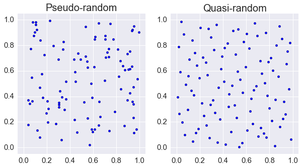
Recall that the convergence of Monte Carlo integration is \(\mathcal{0}(n^{1/2})\). One issue with simple Monte Carlo is that randomly chosen points tend to be clumped. Clumping reduces accuracy since nearby points provide little additional information about the function begin estimated. One way to address this is to split the space into multiple integration regions, then sum them up. This is known as stratified sampling. Another alternative is to use quasi-random numbers which fill space more efficiently than random sequences

It turns out that if we use quasi-random or low discrepancy sequences, we can get convergence approaching \(\mathcal{0}(1/n)\). There are several such generators, but their use in statistical settings is limited to cases where we are integrating with respect to uniform distributions. The regularity can also give rise to errors when estimating integrals of periodic functions. However, these quasi-Monte Carlo methods are used in computational finance models.

Run

! pip install ghalton

if ghalton is not installed.

In [31]:

import ghalton
# create a quasi-random number generator
gen = ghalton.Halton(2)

In [32]:

plt.figure(figsize=(10,5))
plt.subplot(121)
xs = np.random.random((100,2))
plt.scatter(xs[:, 0], xs[:,1])
plt.axis([-0.05, 1.05, -0.05, 1.05])
plt.title('Pseudo-random', fontsize=20)
plt.subplot(122)
ys = np.array(gen.get(100))
plt.scatter(ys[:, 0], ys[:,1])
plt.axis([-0.05, 1.05, -0.05, 1.05])
plt.title('Quasi-random', fontsize=20);

In [33]:

# compute true tail probability of Cauchy distribution
h_true = 1 - stats.cauchy().cdf(3)

In [34]:

# run 5 trails with 10 samples
n = 10
# draw from a uniform distribution
x = stats.uniform().rvs((n, 5))
# evaluate the Cauchy density
y = 3.0/(np.pi * (9 + x**2))
# take average
h_mc = np.sum(y, 0)/n
# display each estimate with its relative error
list(zip(h_mc, 100*np.abs(h_mc - h_true)/h_true))

Out[34]:

[(0.1026491781, 0.2273032411),
 (0.1029048787, 0.4769709316),
 (0.1026105147, 0.1895520269),
 (0.1029257904, 0.4973892209),
 (0.1025694776, 0.1494831832)]

In [35]:

# now use quasi-random samples
gen1 = ghalton.Halton(1)
# generate same number of samples
x = np.reshape(gen1.get(n*5), (n, 5))
# evaluate density
y = 3.0/(np.pi * (9 + x**2))
# take averages
h_qmc = np.sum(y, 0)/n
# print estimate with relative error
list(zip(h_qmc, 100*np.abs(h_qmc - h_true)/h_true))

Out[35]:

[(0.1026632536, 0.2410466633),
 (0.1023042949, 0.1094428682),
 (0.1026741252, 0.2516617574),
 (0.1029118212, 0.4837496311),
 (0.1026111501, 0.1901724534)]

Exercises

Problem 1: Naive MC to Estimate Pi

Part 1: Estimate pi by sampling from the uniform distribution on [-1,1]x[-1,1] using 1000 samples and calculate the relative error |estimate - true|/true

In [36]:

# solution
n = 1000
# sample x coordinates
x_samps = 2*np.random.random(n) - 1
# sample y coordinates
y_samps = 2*np.random.random(n) - 1
# calculate proportion that have distance > 1 from origin
pi_est = 4*np.sum(np.sqrt(x_samps**2 + y_samps**2) < 1)/n
# print results
print("Estimate: ",pi_est)
print("Error: ", np.abs(pi_est - np.pi)/np.pi)

Estimate:  3.08
Error:  0.0196055505539

Part 2: Use on of the MC swindles discussed in this chapter, improve the estimate (still sampling from [-1,1]x[-1,1] and using 1000 samples)

In [37]:

# use this line to intall
#!pip install ghalton
import ghalton
# create a quasi-random number generator
# in 2 dimensions
gen = ghalton.Halton(2)
box_samps = 2*np.array(gen.get(n))
new_samps = box_samps - np.ones_like(box_samps)
pi_est = 4*np.sum(np.sqrt(new_samps[:,0]**2 + new_samps[:,1]**2) < 1)/n
# print results
print("Estimate: ",pi_est)
print("Error: ", np.abs(pi_est - np.pi)/np.pi)

Estimate:  3.148
Error:  0.00203952170657

Problem 2: Importance Sampling

Part 1: For refernce, calculate \(P(X > 3)\) where \(X\) has a standard normal distribution.

In [38]:

import scipy
# calculate tail probability
upper_tail = 1 - scipy.stats.norm.cdf(3)
print(upper_tail)

0.00134989803163

Part 2: Write a function that takes as its arguments a sample size n and a center mu. The function should return a MC estimate of the tail probability calculated above using an importance sampler with a normal proposal with mean mu and variance one.

In [39]:

def gauss_ratio(x, mu):
    return np.exp((mu**2 - 2*mu*x)/2)

def normal_import(n, mu):
    samps = np.random.normal(size = n, loc = mu)
    est = np.mean((samps > 3)*gauss_ratio(samps, mu))
    return est

In [40]:

# test with normal distribution centered at 3
# should give something close to true value
normal_import(1000, 3)

Out[40]:

0.0012728942

Part 3: For 100 values of mu between -10 and 10 calculate 500 estimates of the tail probability with 1000 estimates.

In [41]:

mus = np.linspace(-1, 7, 100)
res_mat = np.empty((500, 100))
for i in range(100):
    for j in range(500):
        res_mat[j,i] = normal_import(1000, mus[i])

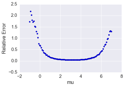
Part 4: For each value of mu plot the average relative error

In [42]:

rel_err = np.abs(res_mat - upper_tail)/upper_tail
col_means = np.mean(rel_err, axis=0)
plt.scatter(mus, col_means)
plt.xlabel("mu")
plt.ylabel("Relative Error")
pass

Part 5: Plot the variance of the estimates for each mu against mu, as above. (It may be interesting to change the y scale to approximately [0,1e-7] to see some details)

In [43]:

col_vars = np.var(res_mat, axis=0)
plt.scatter(mus, col_vars)
plt.ylim((0,2e-7))
plt.xlabel("mu")
plt.ylabel("Variance")

Out[43]:

<matplotlib.text.Text at 0x11c941978>

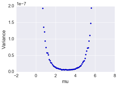
Part 6: Suppose that you were going to pick a value of mu to perform importance sampling. What would be a good choice? What would happen if you made a bad choice?

Picking \(\mu = 3\) would likely minimize the variance and average relative error. Picking \(\mu\) far from 3 would increase the expected relative error and variance of the estimate. This demonstrates how importance sampling can perform poorly if a poor importance distribution is selected.

Part 7: Estimate the tail probability by sampling from the uniform distribution on \([0,1]\) using 1000 samples.

We will use the transformation \(y = 3/x\):

\begin{align} I &= \int_3^\infty \frac{1}{\sqrt{2\pi}}e^{-x^2/2}\,dx \\ &= \int_{3/3}^{3/\infty} \left(-\frac{x^2}{3\sqrt{2\pi}}\right)e^{-\frac{9}{2y^2}}\,dy \\ &= \int_0^1 \left(\frac{3}{y^2\sqrt{2\pi}}\right)e^{-\frac{9}{2y^2}}\,dy. \end{align}

As the uniform density on \([0,1]\) is 1, we can treat this as an expectation over the distribution with no modification.

In [44]:

def f(x):
    val = 3/(x**2*np.sqrt(2*np.pi))*np.exp(-9/(2*x**2))
    return val

samps = np.random.random(size=1000)
est = np.mean(f(samps))
print("Estimate: ",est)
print("True: ", upper_tail)

Estimate:  0.00144386044286
True:  0.00134989803163