Optimization and PCA¶

Question 1 (25 points). Consider the following function on \(\mathbb{R}^2\):

\[f(x_1,x_2) = -x_1x_2e^{-\frac{(x_1^2+x_2^2)}{2}}\]

Use sympy to compute its gradient.
Compute the Hessian matrix.
Find the critical points of \(f\).
Characterize the critical points as max/min or neither.
Find the minimum under the constraint

\[g(x) = x_1^2+x_2^2 \leq 10\]

and

\[ \begin{align}\begin{aligned}h(x) = 2x_1 + 3x_2 = 5\\using ``scipy.optimize.minimize``.\end{aligned}\end{align} \]
Plot the function using matplotlib.

In [ ]:

Question 2 (15 points).

A milkmaid is at point A and needs to get to point B. However, she also needs to fill a pail of water from the river en route from A to B. The equation of the river’s path is shown in the figure below. What is the minimum distance she has to travel to do this?

1. Solve using scipy.optimize and constrained minimization. 2.

Create a plot of the solution using matplotlib (similar to provided figure but with optimal path added).

Note: Beware of local optima.

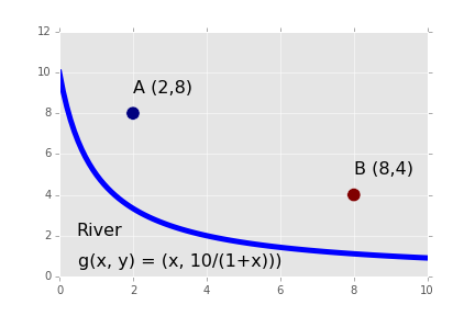
Milkmaid problem

In [ ]:

Background to Q3 - Q5¶

Latent Semantic Analysis (LSA) is a method for reducing the dimnesionality of documents treated as a bag of words. It is used for document classification, clustering and retrieval. For example, LSA can be used to search for prior art given a new patent application. In this homework, we will implement a small library for simple latent semantic analysis as a practical example of the application of SVD. The ideas are very similar to PCA.

We will implement a toy example of LSA to get familiar with the ideas. If you want to use LSA or similar methods for statiscal language analyis, the most efficient Python library is probably gensim - this also provides an online algorithm - i.e. the training information can be continuously updated. Other useful functions for processing natural language can be found in the Natural Lnaguage Toolkit.

Note: The SVD from scipy.linalg performs a full decomposition, which is inefficient since we only need to decompose until we get the first k singluar values. If the SVD from scipy.linalg is too slow, please use the sparsesvd function from the sparsesvd package to perform SVD instead. You can install in the usual way with

!pip install sparsesvd

Then import the following

from sparsesvd import sparsesvd
from scipy.sparse import csc_matrix

and use as follows

sparsesvd(csc_matrix(M), k=10)

Question 3 (20 points): Write 3 functions to calculate the term frequency (tf), the inverse document frequency (idf) and the product (tf-idf). Each function should take a single argument docs, which is a dictionary of (key=identifier, value=dcoument text) pairs, and return an appropriately sized array. Convert ‘-‘ to ‘ ‘ (space), remove punctuation, convert text to lowercase and split on whitespace to generate a collection of terms from the dcoument text.

tf = the number of occurrences of term \(i\) in document \(j\)
idf = \(\log \frac{n}{1 + \text{df}_i}\) where \(n\) is the total number of documents and \(\text{df}_i\) is the number of documents in which term \(i\) occurs.

Print the table of tf-idf values for the following document collection

s1 = "The quick brown fox"
s2 = "Brown fox jumps over the jumps jumps jumps"
s3 = "The the the lazy dog elephant."
s4 = "The the the the the dog peacock lion tiger elephant"

docs = {'s1': s1, 's2': s2, 's3': s3, 's4': s4}

Note: You can use either a numpy array or pandas dataframe to store the matrix. However, we suggest using a Pnadas dataframe since that will allow you to keep track of the row (term) and column (document) names in a single object. Of course, you could also maintain a numpy matrix, a list of terms, and a list of documents separately if you prefer.

In [ ]:

Question 4 (20 points)

Write a function that takes a matrix \(M\) and an integer \(k\) as arguments, and reconstructs a reduced matrix using only the \(k\) largest singular values. Use the scipy.linagl.svd function to perform the decomposition. This is the least squares approximation to the matrix \(M\) in \(k\) dimensions.

Apply the function you just wrote to the following term-frequency matrix for a set of \(9\) documents using \(k=2\) and print the reconstructed matrix \(M'\).

M = np.array([[1, 0, 0, 1, 0, 0, 0, 0, 0],
   [1, 0, 1, 0, 0, 0, 0, 0, 0],
   [1, 1, 0, 0, 0, 0, 0, 0, 0],
   [0, 1, 1, 0, 1, 0, 0, 0, 0],
   [0, 1, 1, 2, 0, 0, 0, 0, 0],
   [0, 1, 0, 0, 1, 0, 0, 0, 0],
   [0, 1, 0, 0, 1, 0, 0, 0, 0],
   [0, 0, 1, 1, 0, 0, 0, 0, 0],
   [0, 1, 0, 0, 0, 0, 0, 0, 1],
   [0, 0, 0, 0, 0, 1, 1, 1, 0],
   [0, 0, 0, 0, 0, 0, 1, 1, 1],
   [0, 0, 0, 0, 0, 0, 0, 1, 1]])

Calculate the pairwise correlation matrix for the original matrix M and the reconstructed matrix using \(k=2\) singular values (you may use scipy.stats.spearmanr to do the calculations). Consider the fist 5 sets of documents as one group \(G1\) and the last 4 as another group \(G2\) (i.e. first 5 and last 4 columns). What is the average within group correlation for \(G1\), \(G2\) and the average cross-group correlation for G1-G2 using either \(M\) or \(M'\). (Do not include self-correlation in the within-group calculations.).

In [ ]:

Question 5 (20 points). Clustering with LSA

Begin by loading a pubmed database of selected article titles using:
```
import pickle
docs = pickle.load(open('pubmed.pic', 'rb'))
```
Create a tf-idf matrix for every term that appears at least once in any of the documents. What is the shape of the tf-idf matrix?
Perform SVD on the tf-idf matrix to obtain \(U \Sigma V^T\) (often written as \(T \Sigma D^T\) in this context with \(T\) representing the terms and \(D\) representing the documents). If we set all but the top \(k\) singular values to 0, the reconstructed matrix is essentially \(U_k \Sigma_k V_k^T\), where \(U_k\) is \(m \times k\), \(\Sigma_k\) is \(k \times k\) and \(V_k^T\) is \(k \times n\). Terms in this reduced space are represented by \(U_k \Sigma_k\) and documents by \(\Sigma_k V^T_k\). Reconstruct the matrix using the first \(k=10\) singular values.
Use agglomerative hierachical clustering with complete linkage to plot a dendrogram and comment on the likely number of document clusters with \(k = 100\). Use the dendrogram function from SciPy.
Determine how similar each of the original documents is to the new document mystery.txt. Since \(A = U \Sigma V^T\), we also have \(V = A^T U S^{-1}\) using orthogonality and the rule for transposing matrix products. This suggests that in order to map the new document to the same concept space, first find the tf-idf vector \(v\) for the new document - this must contain all (and only) the terms present in the existing tf-idx matrix. Then the query vector \(q\) is given by \(v^T U_k \Sigma_k^{-1}\). Find the 10 documents most similar to the new document and the 10 most dissimilar.
Many documents often have some boilerplate material such as organization information, Copyright, etc. at the front or back of the document. Does it matter that the front and back matter of each document is essentially identical for either LSA-based clustering (part 3) or information retrieval (part 4)? Why or why not?

In [1]:

open('mystery.txt')

Out[1]:

<_io.TextIOWrapper name='mystery.txt' mode='r' encoding='UTF-8'>

In [ ]:

Optimization and PCA¶

Background to Q3 - Q5¶

Page contents

This Page