Using `numpy`¶

The foundation for numerical computaiotn in Python is the numpy package, and essentially all scientific libraries in Python build on this - e.g. scipy, pandas, statsmodels, scikit-learn, cv2 etc. The basic data structure in numpy is the NDArray, and it is essential to become familiar with how to slice and dice this object.

Numpy also has the random, and linalg modules that we will discuss in later lectures.

Resources¶

NDArray¶

The base structure in numpy is ndarray, used to represent vectors, matrices and higher-dimensional arrays. Each ndarray has the following attributes:

dtype = correspond to data types in C
shape = dimensionns of array
strides = number of bytes to step in each direction when traversing the array

In [2]:

x = np.array([1,2,3,4,5,6])
print(x)
print('dytpe', x.dtype)
print('shape', x.shape)
print('strides', x.strides)

[1 2 3 4 5 6]
dytpe int64
shape (6,)
strides (8,)

In [3]:

x.shape = (2,3)
print(x)
print('dytpe', x.dtype)
print('shape', x.shape)
print('strides', x.strides)

[[1 2 3]
 [4 5 6]]
dytpe int64
shape (2, 3)
strides (24, 8)

In [4]:

x = x.astype('complex')
print(x)
print('dytpe', x.dtype)
print('shape', x.shape)
print('strides', x.strides)

[[ 1.+0.j  2.+0.j  3.+0.j]
 [ 4.+0.j  5.+0.j  6.+0.j]]
dytpe complex128
shape (2, 3)
strides (48, 16)

Array creation¶

In [5]:

np.array([1,2,3])

Out[5]:

array([1, 2, 3])

In [6]:

np.array([1,2,3], np.float64)

Out[6]:

array([ 1.,  2.,  3.])

In [7]:

np.arange(3)

Out[7]:

array([0, 1, 2])

In [8]:

np.arange(3, 6, 0.5)

Out[8]:

array([ 3. ,  3.5,  4. ,  4.5,  5. ,  5.5])

In [9]:

np.array([[1,2,3],[4,5,6]])

Out[9]:

array([[1, 2, 3],
       [4, 5, 6]])

In [10]:

np.ones(3)

Out[10]:

array([ 1.,  1.,  1.])

In [11]:

np.zeros((3,4))

Out[11]:

array([[ 0.,  0.,  0.,  0.],
       [ 0.,  0.,  0.,  0.],
       [ 0.,  0.,  0.,  0.]])

In [12]:

np.eye(4)

Out[12]:

array([[ 1.,  0.,  0.,  0.],
       [ 0.,  1.,  0.,  0.],
       [ 0.,  0.,  1.,  0.],
       [ 0.,  0.,  0.,  1.]])

In [13]:

np.diag([1,2,3,4])

Out[13]:

array([[1, 0, 0, 0],
       [0, 2, 0, 0],
       [0, 0, 3, 0],
       [0, 0, 0, 4]])

In [14]:

np.fromfunction(lambda i, j: i**2+j**2, (4,5))

Out[14]:

array([[  0.,   1.,   4.,   9.,  16.],
       [  1.,   2.,   5.,  10.,  17.],
       [  4.,   5.,   8.,  13.,  20.],
       [  9.,  10.,  13.,  18.,  25.]])

Array manipulaiton¶

In [15]:

x = np.fromfunction(lambda i, j: i**2+j**2, (4,5))
x

Out[15]:

array([[  0.,   1.,   4.,   9.,  16.],
       [  1.,   2.,   5.,  10.,  17.],
       [  4.,   5.,   8.,  13.,  20.],
       [  9.,  10.,  13.,  18.,  25.]])

In [16]:

x.shape

Out[16]:

(4, 5)

In [17]:

x.size

Out[17]:

In [18]:

x.dtype

Out[18]:

dtype('float64')

In [19]:

x.astype(np.int64)

Out[19]:

array([[ 0,  1,  4,  9, 16],
       [ 1,  2,  5, 10, 17],
       [ 4,  5,  8, 13, 20],
       [ 9, 10, 13, 18, 25]])

In [20]:

x.T

Out[20]:

array([[  0.,   1.,   4.,   9.],
       [  1.,   2.,   5.,  10.],
       [  4.,   5.,   8.,  13.],
       [  9.,  10.,  13.,  18.],
       [ 16.,  17.,  20.,  25.]])

In [21]:

x.reshape(2,-1)

Out[21]:

array([[  0.,   1.,   4.,   9.,  16.,   1.,   2.,   5.,  10.,  17.],
       [  4.,   5.,   8.,  13.,  20.,   9.,  10.,  13.,  18.,  25.]])

Array indexing¶

In [22]:

Out[22]:

array([[  0.,   1.,   4.,   9.,  16.],
       [  1.,   2.,   5.,  10.,  17.],
       [  4.,   5.,   8.,  13.,  20.],
       [  9.,  10.,  13.,  18.,  25.]])

In [23]:

x[0]

Out[23]:

array([  0.,   1.,   4.,   9.,  16.])

In [24]:

x[0,:]

Out[24]:

array([  0.,   1.,   4.,   9.,  16.])

In [25]:

x[:,0]

Out[25]:

array([ 0.,  1.,  4.,  9.])

In [26]:

x[-1]

Out[26]:

array([  9.,  10.,  13.,  18.,  25.])

In [27]:

x[1,1]

Out[27]:

2.0

In [28]:

x[:, 1:3]

Out[28]:

array([[  1.,   4.],
       [  2.,   5.],
       [  5.,   8.],
       [ 10.,  13.]])

Boolkean indexing¶

In [29]:

x >= 2

Out[29]:

array([[False, False,  True,  True,  True],
       [False,  True,  True,  True,  True],
       [ True,  True,  True,  True,  True],
       [ True,  True,  True,  True,  True]], dtype=bool)

In [30]:

x[x > 2]

Out[30]:

array([  4.,   9.,  16.,   5.,  10.,  17.,   4.,   5.,   8.,  13.,  20.,
         9.,  10.,  13.,  18.,  25.])

Fancy indexing¶

In [31]:

x[0, [1,2]]

Out[31]:

array([ 1.,  4.])

Calculations and broadcasting¶

Broadcasting refers to the set of rules that numpy uses to perfrom operations on arrays with differetn shapes. See official documentaiton for a clear explanaiton of the rules. Array shapes can be maniipulated using the reshape method or by inserting a new axis with np.newaxis. Note that np.newaxis is an alias for None, which I sometimes use in my examples.

In [32]:

x = np.fromfunction(lambda i, j: i**2+j**2, (2,3))
x

Out[32]:

array([[ 0.,  1.,  4.],
       [ 1.,  2.,  5.]])

In [33]:

x * 5

Out[33]:

array([[  0.,   5.,  20.],
       [  5.,  10.,  25.]])

In [34]:

x + x

Out[34]:

array([[  0.,   2.,   8.],
       [  2.,   4.,  10.]])

In [35]:

x @ x.T

Out[35]:

array([[ 17.,  22.],
       [ 22.,  30.]])

In [36]:

x.T @ x

Out[36]:

array([[  1.,   2.,   5.],
       [  2.,   5.,  14.],
       [  5.,  14.,  41.]])

In [37]:

np.log1p(x)

Out[37]:

array([[ 0.        ,  0.69314718,  1.60943791],
       [ 0.69314718,  1.09861229,  1.79175947]])

In [38]:

np.exp(x)

Out[38]:

array([[   1.        ,    2.71828183,   54.59815003],
       [   2.71828183,    7.3890561 ,  148.4131591 ]])

Combining and splitting arrays¶

In [39]:

Out[39]:

array([[ 0.,  1.,  4.],
       [ 1.,  2.,  5.]])

In [40]:

np.r_[x, x]

Out[40]:

array([[ 0.,  1.,  4.],
       [ 1.,  2.,  5.],
       [ 0.,  1.,  4.],
       [ 1.,  2.,  5.]])

In [41]:

np.vstack([x, x])

Out[41]:

array([[ 0.,  1.,  4.],
       [ 1.,  2.,  5.],
       [ 0.,  1.,  4.],
       [ 1.,  2.,  5.]])

In [42]:

np.concatenate([x, x], axis=0)

Out[42]:

array([[ 0.,  1.,  4.],
       [ 1.,  2.,  5.],
       [ 0.,  1.,  4.],
       [ 1.,  2.,  5.]])

In [43]:

np.c_[x,x]

Out[43]:

array([[ 0.,  1.,  4.,  0.,  1.,  4.],
       [ 1.,  2.,  5.,  1.,  2.,  5.]])

In [44]:

np.hstack([x, x])

Out[44]:

array([[ 0.,  1.,  4.,  0.,  1.,  4.],
       [ 1.,  2.,  5.,  1.,  2.,  5.]])

In [45]:

np.concatenate([x,x], axis=1)

Out[45]:

array([[ 0.,  1.,  4.,  0.,  1.,  4.],
       [ 1.,  2.,  5.,  1.,  2.,  5.]])

In [46]:

y = np.r_[x, x]
y

Out[46]:

array([[ 0.,  1.,  4.],
       [ 1.,  2.,  5.],
       [ 0.,  1.,  4.],
       [ 1.,  2.,  5.]])

In [47]:

a, b, c = np.hsplit(y, 3)

In [48]:

Out[48]:

array([[ 0.],
       [ 1.],
       [ 0.],
       [ 1.]])

In [49]:

Out[49]:

array([[ 1.],
       [ 2.],
       [ 1.],
       [ 2.]])

In [50]:

Out[50]:

array([[ 4.],
       [ 5.],
       [ 4.],
       [ 5.]])

In [51]:

np.vsplit(y, [3])

Out[51]:

[array([[ 0.,  1.,  4.],
        [ 1.,  2.,  5.],
        [ 0.,  1.,  4.]]), array([[ 1.,  2.,  5.]])]

In [52]:

np.split(y, [3], axis=0)

Out[52]:

[array([[ 0.,  1.,  4.],
        [ 1.,  2.,  5.],
        [ 0.,  1.,  4.]]), array([[ 1.,  2.,  5.]])]

In [53]:

np.hstack(np.hsplit(y, 3))

Out[53]:

array([[ 0.,  1.,  4.],
       [ 1.,  2.,  5.],
       [ 0.,  1.,  4.],
       [ 1.,  2.,  5.]])

Reductions¶

In [54]:

Out[54]:

array([[ 0.,  1.,  4.],
       [ 1.,  2.,  5.],
       [ 0.,  1.,  4.],
       [ 1.,  2.,  5.]])

In [55]:

y.sum()

Out[55]:

26.0

In [56]:

y.sum(0) # column sum

Out[56]:

array([  2.,   6.,  18.])

In [57]:

y.sum(1) # row sum

Out[57]:

array([ 5.,  8.,  5.,  8.])

Standardize by column mean and standard deviation¶

In [58]:

z = (y - y.mean(0))/y.std(0)

In [59]:

Out[59]:

array([[-1., -1., -1.],
       [ 1.,  1.,  1.],
       [-1., -1., -1.],
       [ 1.,  1.,  1.]])

In [60]:

z.mean(0), z.std(0)

Out[60]:

(array([ 0.,  0.,  0.]), array([ 1.,  1.,  1.]))

Standardize by row mean and standard deviation¶

In [61]:

z = (y - y.mean(1)[:,None])/y.std(1)[:,None]

In [62]:

Out[62]:

array([[-0.98058068, -0.39223227,  1.37281295],
       [-0.98058068, -0.39223227,  1.37281295],
       [-0.98058068, -0.39223227,  1.37281295],
       [-0.98058068, -0.39223227,  1.37281295]])

In [63]:

z.mean(1), z.std(1)

Out[63]:

(array([ -7.40148683e-17,   7.40148683e-17,  -7.40148683e-17,
          7.40148683e-17]), array([ 1.,  1.,  1.,  1.]))

Example: Calculating pairwise distance matrix using broadcasting and vectorization¶

Calculate the pairwise distance matrix between the following points

(0,0)
(4,0)
(4,3)
(0,3)

In [64]:

def distance_matrix_py(pts):
    """Returns matrix of pairwise Euclidean distances. Pure Python version."""
    n = len(pts)
    p = len(pts[0])
    m = np.zeros((n, n))
    for i in range(n):
        for j in range(n):
            s = 0
            for k in range(p):
                s += (pts[i,k] - pts[j,k])**2
            m[i, j] = s**0.5
    return m

In [65]:

def distance_matrix_np(pts):
    """Returns matrix of pairwise Euclidean distances. Vectorized numpy version."""
    return np.sum((pts[None,:] - pts[:, None])**2, -1)**0.5

In [66]:

pts = np.array([(0,0), (4,0), (4,3), (0,3)])
pts

Out[66]:

array([[0, 0],
       [4, 0],
       [4, 3],
       [0, 3]])

In [67]:

pts.shape

Out[67]:

(4, 2)

In [68]:

n = pts.shape[0]
p = pts.shape[1]
dist = np.zeros((n, n))
for i in range(n):
    for j in range(n):
        s = 0
        for k in range(p):
            s += (pts[i, k] - pts[j, k])**2
        dist[i, j] = np.sqrt(s)
dist

Out[68]:

array([[ 0.,  4.,  5.,  3.],
       [ 4.,  0.,  3.,  5.],
       [ 5.,  3.,  0.,  4.],
       [ 3.,  5.,  4.,  0.]])

Using broadcasting¶

In [69]:

pts[None, :].shape

Out[69]:

(1, 4, 2)

In [70]:

pts[:, None].shape

Out[70]:

(4, 1, 2)

In [71]:

m = pts[None, :] - pts[:, None]
m

Out[71]:

array([[[ 0,  0],
        [ 4,  0],
        [ 4,  3],
        [ 0,  3]],

       [[-4,  0],
        [ 0,  0],
        [ 0,  3],
        [-4,  3]],

       [[-4, -3],
        [ 0, -3],
        [ 0,  0],
        [-4,  0]],

       [[ 0, -3],
        [ 4, -3],
        [ 4,  0],
        [ 0,  0]]])

In [72]:

m**2

Out[72]:

array([[[ 0,  0],
        [16,  0],
        [16,  9],
        [ 0,  9]],

       [[16,  0],
        [ 0,  0],
        [ 0,  9],
        [16,  9]],

       [[16,  9],
        [ 0,  9],
        [ 0,  0],
        [16,  0]],

       [[ 0,  9],
        [16,  9],
        [16,  0],
        [ 0,  0]]])

In [73]:

(m**2).shape

Out[73]:

(4, 4, 2)

We want to end up with a 4 by 4 matrix, so sum over the axis with dimenion 2. This is axis=2, or axis=-1 since it is the first axis from the end.

In [74]:

np.sum((pts[None, :] - pts[:, None])**2, -1)

Out[74]:

array([[ 0, 16, 25,  9],
       [16,  0,  9, 25],
       [25,  9,  0, 16],
       [ 9, 25, 16,  0]])

Basically, the distance matrix can be calculated in one line of numpy code¶

In [75]:

np.sqrt(np.sum((pts[None, :] - pts[:, None])**2, -1))

Out[75]:

array([[ 0.,  4.,  5.,  3.],
       [ 4.,  0.,  3.,  5.],
       [ 5.,  3.,  0.,  4.],
       [ 3.,  5.,  4.,  0.]])

Let’s put them in funcitons and compare the time.

In [76]:

def pdist1(pts):
    n = pts.shape[0]
    p = pts.shape[1]
    dist = np.zeros((n, n))
    for i in range(n):
        for j in range(n):
            s = 0
            for k in range(p):
                s += (pts[i, k] - pts[j, k])**2
            dist[i, j] = s
    return np.sqrt(dist)

In [77]:

def pdist2(pts):
    return np.sqrt(np.sum((pts[None, :] - pts[:, None])**2, -1))

Check that the outputs are the same¶

In [78]:

np.alltrue(pdist1(pts) == pdist2(pts))

Out[78]:

True

In [79]:

pts = np.random.random((1000, 2))

In [80]:

%timeit pdist1(pts)

1 loops, best of 3: 3.26 s per loop

In [81]:

%timeit pdist2(pts)

10 loops, best of 3: 77.3 ms per loop

But don’t give up on loops yet¶

In [82]:

from numba import njit

In [83]:

@njit
def pdist3(pts):
    n = pts.shape[0]
    p = pts.shape[1]
    dist = np.zeros((n, n))
    for i in range(n):
        for j in range(n):
            s = 0
            for k in range(p):
                s += (pts[i, k] - pts[j, k])**2
            dist[i, j] = s
    return np.sqrt(dist)

In [84]:

%timeit pdist3(pts)

The slowest run took 27.17 times longer than the fastest. This could mean that an intermediate result is being cached
1 loops, best of 3: 16.1 ms per loop

What is going on?¶

This is 3-5 times faster than the broadcasting version! We have just performed Just In Time (JIT) compilation of a function, which will be discussed in a later lecture.

Example: Consructing leave-one-out arrays¶

Another example of numpy trickery is to construct a levae-one-out matrix of a vecotr of length k. In the matrix, each row is a vecotr of length k-1, with a different vector compeont dropped each time. This cna be used for LOOCV to evalaute the out-of-sample accuracy of a predictive model.

For example, suppose you have data points [(1,4), (2,7), (3,11), (4,9), (5,15)] that you want to perfrom LOOCV on for a simple regression model. For each cross-validation, you use one point for testing, and the remainign 4 points for training. In other words, you want the trainigng set to be:

[(2,7), (3,11), (4,9), (5,15)]
[(1,4), (3,11), (4,9), (5,15)]
[(1,4), (2,7),  (4,9), (5,15)]
[(1,4), (2,7), (3,11), (5,15)]
[(1,4), (2,7), (3,11), (4,9)]

Here is one way to do create the training set using numpy tricks.

Create a triangular matrix with N rows, N-1 columns and offset from diagnonal by -1

In [85]:

N = 5

In [86]:

np.tri(N)

Out[86]:

array([[ 1.,  0.,  0.,  0.,  0.],
       [ 1.,  1.,  0.,  0.,  0.],
       [ 1.,  1.,  1.,  0.,  0.],
       [ 1.,  1.,  1.,  1.,  0.],
       [ 1.,  1.,  1.,  1.,  1.]])

In [87]:

np.tri(N, N-1)

Out[87]:

array([[ 1.,  0.,  0.,  0.],
       [ 1.,  1.,  0.,  0.],
       [ 1.,  1.,  1.,  0.],
       [ 1.,  1.,  1.,  1.],
       [ 1.,  1.,  1.,  1.]])

In [88]:

np.tri(N, N-1, -1)

Out[88]:

array([[ 0.,  0.,  0.,  0.],
       [ 1.,  0.,  0.,  0.],
       [ 1.,  1.,  0.,  0.],
       [ 1.,  1.,  1.,  0.],
       [ 1.,  1.,  1.,  1.]])

Use broadcasting to create a new index matrix

In [89]:

np.arange(1, N)

Out[89]:

array([1, 2, 3, 4])

In [90]:

np.arange(1, N) - np.tri(N, N-1, -1)

Out[90]:

array([[ 1.,  2.,  3.,  4.],
       [ 0.,  2.,  3.,  4.],
       [ 0.,  1.,  3.,  4.],
       [ 0.,  1.,  2.,  4.],
       [ 0.,  1.,  2.,  3.]])

In [91]:

idx = np.arange(1, N) - np.tri(N, N-1, -1).astype('int')

In [92]:

data = np.array([(1,4), (2,7), (3,11), (4,9), (5,15)])
data

Out[92]:

array([[ 1,  4],
       [ 2,  7],
       [ 3, 11],
       [ 4,  9],
       [ 5, 15]])

In [93]:

data[idx]

Out[93]:

array([[[ 2,  7],
        [ 3, 11],
        [ 4,  9],
        [ 5, 15]],

       [[ 1,  4],
        [ 3, 11],
        [ 4,  9],
        [ 5, 15]],

       [[ 1,  4],
        [ 2,  7],
        [ 4,  9],
        [ 5, 15]],

       [[ 1,  4],
        [ 2,  7],
        [ 3, 11],
        [ 5, 15]],

       [[ 1,  4],
        [ 2,  7],
        [ 3, 11],
        [ 4,  9]]])

All but one¶

R uses negative indexing to mena delete the component at that index. Because Python uses negative indexing to mean count from the end, we have to do a little more work to get the same effect. Here are two ways of deleting one item from a vector.

In [94]:

def f1(a, k):
    idx = np.ones_like(a).astype('bool')
    idx[k] = 0
    return a[idx]

In [95]:

def f2(a, k):
    return np.r_[a[:k], a[k+1:]]

In [96]:

a = np.arange(100)
k = 50

In [97]:

%timeit f1(a, k)

The slowest run took 6.39 times longer than the fastest. This could mean that an intermediate result is being cached
100000 loops, best of 3: 12.4 µs per loop

In [98]:

%timeit f2(a, k)

10000 loops, best of 3: 47.6 µs per loop

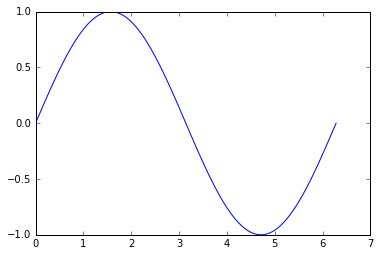
Universal functions (Ufuncs)¶

Functions that work on both scalars and arrays are known as ufuncs. For arrays, ufuncs apply the function in an element-wise fashion. Use of ufuncs is an esssential aspect of vectorization and typically much more computtionally efficient than using an explicit loop over each element.

In [99]:

import matplotlib.pyplot as plt
%matplotlib inline

xs = np.linspace(0, 2*np.pi, 100)
ys = np.sin(xs) # np.sin is a universal function
plt.plot(xs, ys);

Generalized ufucns¶

A universal function performs vectorized looping over scalars. A generalized ufucn performs looping over vectors or arrays. Currently, numpy only ships with a single generalized ufunc. However, they play an important role for JIT compilation with numba, a topic we will cover in future lectures.

In [100]:

from numpy.core.umath_tests import matrix_multiply

print(matrix_multiply.signature)

(m,n),(n,p)->(m,p)

In [101]:

us = np.random.random((5, 2, 3)) # 5 2x3 matrics
vs = np.random.random((5, 3, 4)) # 5 3x4 matrices

In [102]:

us

Out[102]:

array([[[ 0.45041464,  0.73156889,  0.20199586],
        [ 0.07597661,  0.13069672,  0.57386177]],

       [[ 0.10830059,  0.26695388,  0.44054188],
        [ 0.57974703,  0.17978862,  0.52472549]],

       [[ 0.40794462,  0.35751635,  0.36870809],
        [ 0.63494551,  0.11960905,  0.51381859]],

       [[ 0.49510212,  0.46783668,  0.07856113],
        [ 0.28401281,  0.47199107,  0.54560703]],

       [[ 0.79458848,  0.43756637,  0.06759583],
        [ 0.40228528,  0.50838122,  0.56375008]]])

In [103]:

vs

Out[103]:

array([[[  5.12266952e-02,   8.40637879e-01,   2.38644940e-01,
           4.35712252e-01],
        [  7.81217918e-01,   6.77203544e-01,   7.28623630e-01,
           8.70980358e-02],
        [  9.53278422e-01,   6.57880491e-01,   4.45387233e-01,
           5.54732924e-02]],

       [[  6.52946888e-01,   2.29030756e-01,   5.91273241e-01,
           8.29711164e-06],
        [  5.25251656e-01,   5.06625358e-01,   1.87996526e-01,
           3.57795468e-02],
        [  6.45830540e-01,   7.67992588e-01,   3.53764451e-01,
           8.93663158e-01]],

       [[  7.05223217e-01,   5.68551438e-01,   2.21699577e-01,
           3.66118249e-01],
        [  3.59834031e-01,   8.86827366e-01,   8.90595276e-01,
           9.32417623e-01],
        [  9.20454420e-01,   8.21082903e-01,   9.46367477e-01,
           6.79992096e-02]],

       [[  5.17735631e-01,   7.57666718e-01,   9.76354847e-01,
           8.23073506e-01],
        [  9.12873687e-01,   7.01160089e-01,   9.41861241e-01,
           5.75122377e-01],
        [  4.29768204e-01,   6.52651201e-01,   4.52733332e-01,
           7.76359616e-01]],

       [[  3.29293395e-01,   6.01805518e-01,   8.82878227e-01,
           9.58704548e-01],
        [  1.57352491e-01,   8.34085919e-01,   2.60621284e-01,
           1.61751295e-01],
        [  1.81993190e-01,   3.98928140e-01,   1.31517889e-01,
           4.99537484e-03]]])

In [104]:

# perform matrix multiplication for each of the 5 sets of matrices
ws = matrix_multiply(us, vs)

In [105]:

ws.shape

Out[105]:

(5, 2, 4)

In [106]:

ws

Out[106]:

array([[[ 0.78714627,  1.00694579,  0.73049393,  0.27117477],
        [ 0.65304469,  0.52990956,  0.36895086,  0.07632137]],

       [[ 0.4954479 ,  0.49838267,  0.2700697 ,  0.40324843],
        [ 0.81186204,  0.62685067,  0.56221777,  0.47536541]],

       [[ 0.75571755,  0.85173269,  0.75777686,  0.50778237],
        [ 0.96376431,  0.88895942,  0.73355161,  0.37892998]],

       [[ 0.71717088,  0.75442382,  0.95959983,  0.73756047],
        [ 0.81239634,  0.90221944,  0.96886187,  0.92880331]],

       [[ 0.34280688,  0.87012156,  0.82445404,  0.83289018],
        [ 0.31506361,  0.89102688,  0.5618071 ,  0.47072019]]])

Saving and loading NDArrays¶

Saving to and loading from text files¶

In [108]:

x1 = np.arange(1,10).reshape(3,3)
x1

Out[108]:

array([[1, 2, 3],
       [4, 5, 6],
       [7, 8, 9]])

In [110]:

np.savetxt('../data/x1.txt', x1)

In [111]:

!cat ../data/x1.txt

1.000000000000000000e+00 2.000000000000000000e+00 3.000000000000000000e+00
4.000000000000000000e+00 5.000000000000000000e+00 6.000000000000000000e+00
7.000000000000000000e+00 8.000000000000000000e+00 9.000000000000000000e+00

In [112]:

x2 = np.loadtxt('../data/x1.txt')
x2

Out[112]:

array([[ 1.,  2.,  3.],
       [ 4.,  5.,  6.],
       [ 7.,  8.,  9.]])

Saving to and loading from binary files (much faster and also preserves dtype)¶

In [115]:

np.save('../data/x1.npy', x1)

In [116]:

!cat ../data/x1.npy

�NUMPYF{'descr': '<i8', 'fortran_order': False, 'shape': (3, 3), }

In [117]:

x3 = np.load('../data/x1.npy')
x3

Out[117]:

array([[1, 2, 3],
       [4, 5, 6],
       [7, 8, 9]])

Version information¶

In [107]:

%load_ext version_information
%version_information numpy, numba, matplotlib

Out[107]:

Software	Version
Python	3.5.1 64bit [GCC 4.2.1 (Apple Inc. build 5577)]
IPython	4.0.1
OS	Darwin 15.2.0 x86_64 i386 64bit
numpy	1.10.2
numba	0.22.1
matplotlib	1.5.1
Fri Jan 15 13:34:06 2016 EST

In [ ]:

Using `numpy`¶

Resources¶

NDArray¶

Array creation¶

Array manipulaiton¶

Array indexing¶

Boolkean indexing¶

Fancy indexing¶

Calculations and broadcasting¶

Combining and splitting arrays¶

Reductions¶

Standardize by column mean and standard deviation¶

Standardize by row mean and standard deviation¶

Example: Calculating pairwise distance matrix using broadcasting and vectorization¶

Using broadcasting¶

Basically, the distance matrix can be calculated in one line of numpy code¶

Check that the outputs are the same¶

But don’t give up on loops yet¶

What is going on?¶

Example: Consructing leave-one-out arrays¶

All but one¶

Universal functions (Ufuncs)¶

Generalized ufucns¶

Saving and loading NDArrays¶

Saving to and loading from text files¶

Saving to and loading from binary files (much faster and also preserves dtype)¶

Version information¶

Page contents

Previous page

Next page

This Page

Using numpy¶

Resources¶

NDArray¶

Array creation¶

Array manipulaiton¶

Array indexing¶

Boolkean indexing¶

Fancy indexing¶

Calculations and broadcasting¶

Combining and splitting arrays¶

Reductions¶

Standardize by column mean and standard deviation¶

Standardize by row mean and standard deviation¶

Example: Calculating pairwise distance matrix using broadcasting and vectorization¶

Using broadcasting¶

Basically, the distance matrix can be calculated in one line of numpy code¶

Check that the outputs are the same¶

But don’t give up on loops yet¶

What is going on?¶

Example: Consructing leave-one-out arrays¶

All but one¶

Universal functions (Ufuncs)¶

Generalized ufucns¶

Saving and loading NDArrays¶

Saving to and loading from text files¶

Saving to and loading from binary files (much faster and also preserves dtype)¶

Version information¶

Using `numpy`¶