Data
Resources
In [1]:
import numpy as np
import pandas as pd
from pandas import Series, DataFrame
import matplotlib.pyplot as plt
%matplotlib inline
In [2]:
plt.style.use('ggplot')
Working with Series
In [3]:
x = Series(range(5,10))
In [4]:
x
Out[4]:
0    5
1    6
2    7
3    8
4    9
dtype: int64
We cna treat Series objects much like numpy vectors
In [5]:
x.sum(), x.mean(), x.std()
Out[5]:
(35, 7.0, 1.5811388300841898)
In [6]:
x**2
Out[6]:
0    25
1    36
2    49
3    64
4    81
dtype: int64
In [7]:
x[x >= 8]
Out[7]:
3    8
4    9
dtype: int64
Series can also contain more information than numpy vectors
Series index
But you can also assign labeled indexes.
In [9]:
x.index = list('abcde')
x
Out[9]:
a    5
b    6
c    7
d    8
e    9
dtype: int64
Note that with labels, the end index is included
In [10]:
x['a':'c']
Out[10]:
a    5
b    6
c    7
dtype: int64
Even when you have a labeled index, positional arguments still work
In [11]:
x[1:4]
Out[11]:
b    6
c    7
d    8
dtype: int64
In [12]:
x.a, x.c, x.e
Out[12]:
(5, 7, 9)
Working with missing data
Missing data is indicated with NaN (not a number).
In [13]:
y = Series([10, np.nan, np.nan, 13, 14])
y
Out[13]:
0    10
1   NaN
2   NaN
3    13
4    14
dtype: float64
Concatenating two series
In [14]:
z = pd.concat([x, y])
z
Out[14]:
a     5
b     6
c     7
d     8
e     9
0    10
1   NaN
2   NaN
3    13
4    14
dtype: float64
Reset index to default
In [15]:
z = z.reset_index(drop=True)
z
Out[15]:
0     5
1     6
2     7
3     8
4     9
5    10
6   NaN
7   NaN
8    13
9    14
dtype: float64
pandas aggregate functions ignore missing data
In [16]:
z.sum(), z.mean(), z.std()
Out[16]:
(72.0, 9.0, 3.2071349029490928)
Selecting non-missing values
In [18]:
z[z.notnull()]
Out[18]:
0     5
1     6
2     7
3     8
4     9
5    10
8    13
9    14
dtype: float64
Replacement of missing values
In [19]:
z.fillna(0)
Out[19]:
0     5
1     6
2     7
3     8
4     9
5    10
6     0
7     0
8    13
9    14
dtype: float64
In [20]:
z.fillna(method='ffill')
Out[20]:
0     5
1     6
2     7
3     8
4     9
5    10
6    10
7    10
8    13
9    14
dtype: float64
In [21]:
z.fillna(method='bfill')
Out[21]:
0     5
1     6
2     7
3     8
4     9
5    10
6    13
7    13
8    13
9    14
dtype: float64
In [22]:
z.fillna(z.mean())
Out[22]:
0     5
1     6
2     7
3     8
4     9
5    10
6     9
7     9
8    13
9    14
dtype: float64
Working with dates / times
We will see more date/time handling in the DataFrame section.
In [23]:
z.index = pd.date_range('01-Jan-2016', periods=len(z))
In [24]:
z
Out[24]:
2016-01-01     5
2016-01-02     6
2016-01-03     7
2016-01-04     8
2016-01-05     9
2016-01-06    10
2016-01-07   NaN
2016-01-08   NaN
2016-01-09    13
2016-01-10    14
Freq: D, dtype: float64
Intelligent aggregation over datetime ranges
In [25]:
z.resample('W', how='sum')
Out[25]:
2016-01-03    18
2016-01-10    54
Freq: W-SUN, dtype: float64
Formatting datetime objects (see http://strftime.org)
In [26]:
z.index.strftime('%b %d, %Y')
Out[26]:
array(['Jan 01, 2016', 'Jan 02, 2016', 'Jan 03, 2016', 'Jan 04, 2016',
       'Jan 05, 2016', 'Jan 06, 2016', 'Jan 07, 2016', 'Jan 08, 2016',
       'Jan 09, 2016', 'Jan 10, 2016'],
      dtype='<U12')
DataFrame
Similar to R.
Titanic data
In [27]:
url = 'https://raw.githubusercontent.com/mwaskom/seaborn-data/master/titanic.csv'
titanic = pd.read_csv(url)
In [28]:
titanic.shape
Out[28]:
(891, 15)
In [29]:
titanic.columns
Out[29]:
Index(['survived', 'pclass', 'sex', 'age', 'sibsp', 'parch', 'fare',
       'embarked', 'class', 'who', 'adult_male', 'deck', 'embark_town',
       'alive', 'alone'],
      dtype='object')
In [30]:
# For display purposes, we will drop some columns
titanic = titanic[['survived', 'sex', 'age', 'fare',
                   'embarked', 'class', 'who', 'deck', 'embark_town',]]
In [31]:
titanic.dtypes
Out[31]:
survived         int64
sex             object
age            float64
fare           float64
embarked        object
class           object
who             object
deck            object
embark_town     object
dtype: object
But I really want to see all the data!
In [32]:
import qgrid
qgrid.nbinstall(overwrite=True)
In [33]:
qgrid.show_grid(titanic)
Summarizing a data frame
In [34]:
titanic.ix[0]
Out[34]:
survived                 0
sex                   male
age                     22
fare                  7.25
embarked                 S
class                Third
who                    man
deck                   NaN
embark_town    Southampton
Name: 0, dtype: object
In [35]:
titanic.describe()
Out[35]:
| survived | age | fare | |
|---|---|---|---|
| count | 891.000000 | 714.000000 | 891.000000 |
| mean | 0.383838 | 29.699118 | 32.204208 |
| std | 0.486592 | 14.526497 | 49.693429 |
| min | 0.000000 | 0.420000 | 0.000000 |
| 25% | 0.000000 | 20.125000 | 7.910400 |
| 50% | 0.000000 | 28.000000 | 14.454200 |
| 75% | 1.000000 | 38.000000 | 31.000000 |
| max | 1.000000 | 80.000000 | 512.329200 |
In [36]:
titanic.head()
Out[36]:
| survived | sex | age | fare | embarked | class | who | deck | embark_town | |
|---|---|---|---|---|---|---|---|---|---|
| 0 | 0 | male | 22 | 7.2500 | S | Third | man | NaN | Southampton |
| 1 | 1 | female | 38 | 71.2833 | C | First | woman | C | Cherbourg |
| 2 | 1 | female | 26 | 7.9250 | S | Third | woman | NaN | Southampton |
| 3 | 1 | female | 35 | 53.1000 | S | First | woman | C | Southampton |
| 4 | 0 | male | 35 | 8.0500 | S | Third | man | NaN | Southampton |
In [37]:
titanic.tail()
Out[37]:
| survived | sex | age | fare | embarked | class | who | deck | embark_town | |
|---|---|---|---|---|---|---|---|---|---|
| 886 | 0 | male | 27 | 13.00 | S | Second | man | NaN | Southampton |
| 887 | 1 | female | 19 | 30.00 | S | First | woman | B | Southampton |
| 888 | 0 | female | NaN | 23.45 | S | Third | woman | NaN | Southampton |
| 889 | 1 | male | 26 | 30.00 | C | First | man | C | Cherbourg |
| 890 | 0 | male | 32 | 7.75 | Q | Third | man | NaN | Queenstown |
In [38]:
titanic.columns
Out[38]:
Index(['survived', 'sex', 'age', 'fare', 'embarked', 'class', 'who', 'deck',
       'embark_town'],
      dtype='object')
In [39]:
titanic.index
Out[39]:
Int64Index([  0,   1,   2,   3,   4,   5,   6,   7,   8,   9,
            ...
            881, 882, 883, 884, 885, 886, 887, 888, 889, 890],
           dtype='int64', length=891)
Indexing
In [40]:
titanic[['sex', 'age', 'class']].head()
Out[40]:
| sex | age | class | |
|---|---|---|---|
| 0 | male | 22 | Third |
| 1 | female | 38 | First |
| 2 | female | 26 | Third |
| 3 | female | 35 | First |
| 4 | male | 35 | Third |
In [41]:
titanic[10:15]
Out[41]:
| survived | sex | age | fare | embarked | class | who | deck | embark_town | |
|---|---|---|---|---|---|---|---|---|---|
| 10 | 1 | female | 4 | 16.7000 | S | Third | child | G | Southampton |
| 11 | 1 | female | 58 | 26.5500 | S | First | woman | C | Southampton |
| 12 | 0 | male | 20 | 8.0500 | S | Third | man | NaN | Southampton |
| 13 | 0 | male | 39 | 31.2750 | S | Third | man | NaN | Southampton |
| 14 | 0 | female | 14 | 7.8542 | S | Third | child | NaN | Southampton |
Using the ix helper for indexing
In [42]:
titanic.ix[10:15, 'age':'fare']
Out[42]:
| age | fare | |
|---|---|---|
| 10 | 4 | 16.7000 |
| 11 | 58 | 26.5500 |
| 12 | 20 | 8.0500 |
| 13 | 39 | 31.2750 |
| 14 | 14 | 7.8542 |
| 15 | 55 | 16.0000 |
In [43]:
titanic.ix[10:15, [1,3,5]]
Out[43]:
| sex | fare | class | |
|---|---|---|---|
| 10 | female | 16.7000 | Third |
| 11 | female | 26.5500 | First |
| 12 | male | 8.0500 | Third |
| 13 | male | 31.2750 | Third |
| 14 | female | 7.8542 | Third |
| 15 | female | 16.0000 | Second |
In [44]:
titanic[titanic.age < 2]
Out[44]:
| survived | sex | age | fare | embarked | class | who | deck | embark_town | |
|---|---|---|---|---|---|---|---|---|---|
| 78 | 1 | male | 0.83 | 29.0000 | S | Second | child | NaN | Southampton |
| 164 | 0 | male | 1.00 | 39.6875 | S | Third | child | NaN | Southampton |
| 172 | 1 | female | 1.00 | 11.1333 | S | Third | child | NaN | Southampton |
| 183 | 1 | male | 1.00 | 39.0000 | S | Second | child | F | Southampton |
| 305 | 1 | male | 0.92 | 151.5500 | S | First | child | C | Southampton |
| 381 | 1 | female | 1.00 | 15.7417 | C | Third | child | NaN | Cherbourg |
| 386 | 0 | male | 1.00 | 46.9000 | S | Third | child | NaN | Southampton |
| 469 | 1 | female | 0.75 | 19.2583 | C | Third | child | NaN | Cherbourg |
| 644 | 1 | female | 0.75 | 19.2583 | C | Third | child | NaN | Cherbourg |
| 755 | 1 | male | 0.67 | 14.5000 | S | Second | child | NaN | Southampton |
| 788 | 1 | male | 1.00 | 20.5750 | S | Third | child | NaN | Southampton |
| 803 | 1 | male | 0.42 | 8.5167 | C | Third | child | NaN | Cherbourg |
| 827 | 1 | male | 1.00 | 37.0042 | C | Second | child | NaN | Cherbourg |
| 831 | 1 | male | 0.83 | 18.7500 | S | Second | child | NaN | Southampton |
Sorting and ordering data
In [45]:
titanic.sort_index().head()
Out[45]:
| survived | sex | age | fare | embarked | class | who | deck | embark_town | |
|---|---|---|---|---|---|---|---|---|---|
| 0 | 0 | male | 22 | 7.2500 | S | Third | man | NaN | Southampton |
| 1 | 1 | female | 38 | 71.2833 | C | First | woman | C | Cherbourg |
| 2 | 1 | female | 26 | 7.9250 | S | Third | woman | NaN | Southampton |
| 3 | 1 | female | 35 | 53.1000 | S | First | woman | C | Southampton |
| 4 | 0 | male | 35 | 8.0500 | S | Third | man | NaN | Southampton |
In [46]:
titanic.sort_values('age', ascending=True).head()
Out[46]:
| survived | sex | age | fare | embarked | class | who | deck | embark_town | |
|---|---|---|---|---|---|---|---|---|---|
| 803 | 1 | male | 0.42 | 8.5167 | C | Third | child | NaN | Cherbourg |
| 755 | 1 | male | 0.67 | 14.5000 | S | Second | child | NaN | Southampton |
| 644 | 1 | female | 0.75 | 19.2583 | C | Third | child | NaN | Cherbourg |
| 469 | 1 | female | 0.75 | 19.2583 | C | Third | child | NaN | Cherbourg |
| 78 | 1 | male | 0.83 | 29.0000 | S | Second | child | NaN | Southampton |
In [47]:
titanic.sort_values(['survived', 'age'], ascending=[True, True]).head()
Out[47]:
| survived | sex | age | fare | embarked | class | who | deck | embark_town | |
|---|---|---|---|---|---|---|---|---|---|
| 164 | 0 | male | 1 | 39.6875 | S | Third | child | NaN | Southampton |
| 386 | 0 | male | 1 | 46.9000 | S | Third | child | NaN | Southampton |
| 7 | 0 | male | 2 | 21.0750 | S | Third | child | NaN | Southampton |
| 16 | 0 | male | 2 | 29.1250 | Q | Third | child | NaN | Queenstown |
| 119 | 0 | female | 2 | 31.2750 | S | Third | child | NaN | Southampton |
Grouping data
In [48]:
sex_class = titanic.groupby(['sex', 'class'])
In [49]:
sex_class.count()
Out[49]:
| survived | age | fare | embarked | who | deck | embark_town | ||
|---|---|---|---|---|---|---|---|---|
| sex | class | |||||||
| female | First | 94 | 85 | 94 | 92 | 94 | 81 | 92 |
| Second | 76 | 74 | 76 | 76 | 76 | 10 | 76 | |
| Third | 144 | 102 | 144 | 144 | 144 | 6 | 144 | |
| male | First | 122 | 101 | 122 | 122 | 122 | 94 | 122 |
| Second | 108 | 99 | 108 | 108 | 108 | 6 | 108 | |
| Third | 347 | 253 | 347 | 347 | 347 | 6 | 347 |
Why Kate Winslett survived and Leonardo DiCaprio didn’t
In [50]:
df = sex_class.mean()
df['survived']
Out[50]:
sex     class
female  First     0.968085
        Second    0.921053
        Third     0.500000
male    First     0.368852
        Second    0.157407
        Third     0.135447
Name: survived, dtype: float64
Of the females who were in first class, count the number from each embarking town
In [51]:
sex_class.get_group(('female', 'First')).groupby('embark_town').count()
Out[51]:
| survived | sex | age | fare | embarked | class | who | deck | |
|---|---|---|---|---|---|---|---|---|
| embark_town | ||||||||
| Cherbourg | 43 | 43 | 38 | 43 | 43 | 43 | 43 | 35 |
| Queenstown | 1 | 1 | 1 | 1 | 1 | 1 | 1 | 1 |
| Southampton | 48 | 48 | 44 | 48 | 48 | 48 | 48 | 43 |
Cross-tabulation
In [52]:
pd.crosstab(titanic.survived, titanic['class'])
Out[52]:
| class | First | Second | Third |
|---|---|---|---|
| survived | |||
| 0 | 80 | 97 | 372 |
| 1 | 136 | 87 | 119 |
We can aslo get multiple summaries at the same time
In [53]:
def my_func(x):
    return np.max(x)
In [54]:
mapped_funcs = {'embarked': 'count', 'age': ('mean', 'median', my_func), 'survived': sum}
sex_class.get_group(('female', 'First')).groupby('embark_town').agg(mapped_funcs)
Out[54]:
| embarked | survived | age | |||
|---|---|---|---|---|---|
| count | sum | mean | median | my_func | |
| embark_town | |||||
| Cherbourg | 43 | 42 | 36.052632 | 37 | 60 |
| Queenstown | 1 | 1 | 33.000000 | 33 | 33 |
| Southampton | 48 | 46 | 32.704545 | 33 | 63 |
In [55]:
titanic.columns
Out[55]:
Index(['survived', 'sex', 'age', 'fare', 'embarked', 'class', 'who', 'deck',
       'embark_town'],
      dtype='object')
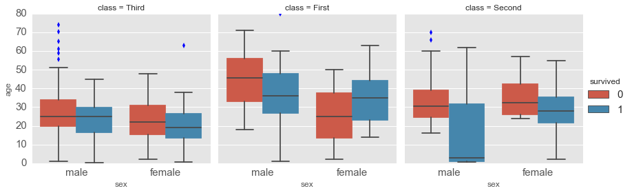
Visualizing tables
See more examples in the Graphics notebook.
In [56]:
import seaborn as sns
sns.set_context(font_scale=4)
sns.factorplot(x='sex', y='age', hue='survived', col='class', kind='box', data=titanic)
pass
/Users/cliburn/anaconda/envs/py35/lib/python3.5/site-packages/matplotlib/__init__.py:892: UserWarning: axes.color_cycle is deprecated and replaced with axes.prop_cycle; please use the latter.
  warnings.warn(self.msg_depr % (key, alt_key))
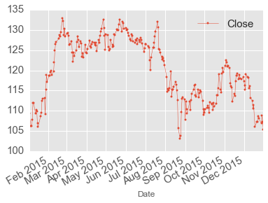
Making plots with pandas
In [57]:
from pandas_datareader import data as web
import datetime
In [58]:
apple = web.DataReader('AAPL', 'google',
                        start = datetime.datetime(2015, 1, 1),
                        end = datetime.datetime(2015, 12, 31))
In [59]:
apple.head()
Out[59]:
| Open | High | Low | Close | Volume | |
|---|---|---|---|---|---|
| Date | |||||
| 2015-01-02 | 111.39 | 111.44 | 107.35 | 109.33 | 53204626 |
| 2015-01-05 | 108.29 | 108.65 | 105.41 | 106.25 | 64285491 |
| 2015-01-06 | 106.54 | 107.43 | 104.63 | 106.26 | 65797116 |
| 2015-01-07 | 107.20 | 108.20 | 106.70 | 107.75 | 40105934 |
| 2015-01-08 | 109.23 | 112.15 | 108.70 | 111.89 | 59364547 |
In [60]:
apple.plot.line(y='Close', marker='o', markersize=3, linewidth=0.5)
pass
In [61]:
# Zoom in on large drop in August
aug = apple['2015-08-01':'2015-08-30']
aug.plot.line(y=['High', 'Low', 'Open', 'Close'], marker='o', markersize=10, linewidth=1)
pass

Data conversions
One of the nicest features of pnadas is the ease of convertign
tabular data across differnt storage formats. We will illustrate by
converting the titanic dataframe into multiple formats.
In [62]:
titanic.head(2)
Out[62]:
| survived | sex | age | fare | embarked | class | who | deck | embark_town | |
|---|---|---|---|---|---|---|---|---|---|
| 0 | 0 | male | 22 | 7.2500 | S | Third | man | NaN | Southampton |
| 1 | 1 | female | 38 | 71.2833 | C | First | woman | C | Cherbourg |
In [63]:
titanic.to_csv('../data/titanic.csv', index=False)
In [64]:
t1 = pd.read_csv('../data/titanic.csv')
t1.head(2)
Out[64]:
| survived | sex | age | fare | embarked | class | who | deck | embark_town | |
|---|---|---|---|---|---|---|---|---|---|
| 0 | 0 | male | 22 | 7.2500 | S | Third | man | NaN | Southampton |
| 1 | 1 | female | 38 | 71.2833 | C | First | woman | C | Cherbourg |
In [65]:
t1.to_excel('../data/titanic.xlsx')
In [66]:
t2 = pd.read_excel('../data/titanic.xlsx')
t2.head(2)
Out[66]:
| survived | sex | age | fare | embarked | class | who | deck | embark_town | |
|---|---|---|---|---|---|---|---|---|---|
| 0 | 0 | male | 22 | 7.2500 | S | Third | man | NaN | Southampton |
| 1 | 1 | female | 38 | 71.2833 | C | First | woman | C | Cherbourg |
In [68]:
import sqlite3

con = sqlite3.connect('../data/titanic.db')
t2.to_sql('titanic', con, index=False, if_exists='replace')
In [69]:
t3 = pd.read_sql('select * from titanic', con)
t3.head(2)
Out[69]:
| survived | sex | age | fare | embarked | class | who | deck | embark_town | |
|---|---|---|---|---|---|---|---|---|---|
| 0 | 0 | male | 22 | 7.2500 | S | Third | man | None | Southampton |
| 1 | 1 | female | 38 | 71.2833 | C | First | woman | C | Cherbourg |
In [70]:
t3.to_json('../data/titanic.json')
In [71]:
t4 = pd.read_json('../data/titanic.json')
t4.head(2)
Out[71]:
| age | class | deck | embark_town | embarked | fare | sex | survived | who | |
|---|---|---|---|---|---|---|---|---|---|
| 0 | 22 | Third | None | Southampton | S | 7.2500 | male | 0 | man |
| 1 | 38 | First | C | Cherbourg | C | 71.2833 | female | 1 | woman |
In [72]:
t4 = t4[t3.columns]
t4.head(2)
Out[72]:
| survived | sex | age | fare | embarked | class | who | deck | embark_town | |
|---|---|---|---|---|---|---|---|---|---|
| 0 | 0 | male | 22 | 7.2500 | S | Third | man | None | Southampton |
| 1 | 1 | female | 38 | 71.2833 | C | First | woman | C | Cherbourg |
Version information
In [73]:
%load_ext version_information
%version_information numpy, pandas, seaborn
Out[73]:
| Software | Version |
|---|---|
| Python | 3.5.1 64bit [GCC 4.2.1 (Apple Inc. build 5577)] |
| IPython | 4.0.1 |
| OS | Darwin 15.2.0 x86_64 i386 64bit |
| numpy | 1.10.4 |
| pandas | 0.17.1 |
| seaborn | 0.6.0 |
| Tue Jan 26 11:59:51 2016 EST | |
In [ ]: