Homework 03
Write code to solve all problems. The grading rubric includes the following criteria:
- Correctness
- Readability
- Efficiency
Please do not copy answers found on the web or elsewhere as it will not benefit your learning. Searching the web for general references etc is OK. Some discussion with friends is fine too - but again, do not just copy their answer.
Honor Code: By submitting this assignment, you certify that this is your original work.
Note: These exercises will involve quite a bit more code writing than the first 2 homework assignments so start early. They are also intentionally less specific so that you have to come up with your own plan to complete the exercises.
We will use the following data sets:
titanic = sns.load_dataset("titanic")
iris = sns.load_dataset("iris")
Q1 (20 pts) Working with numpy.random.
Part 1 (10 pts) Consider a sequence of \(n\) Bernoulli trials with success probabilty \(p\) per trial. A string of consecutive successes is known as a success run. Write a function that returns the counts for runs of length \(k\) for each \(k\) observed in a dictionary.
For example: if the trials were [0, 1, 0, 1, 1, 0, 0, 0, 0, 1], the function should return
{1: 2, 2: 1})
In [41]:
from collections import Counter

def count_runs(xs):
    """Count number of success runs of length k."""
    ys = []
    count = 0
    for x in xs:
        if x == 1:
            count += 1
        else:
            if count: ys.append(count)
            count = 0
    if count: ys.append(count)
    return Counter(ys)
In [42]:
count_runs([0, 1, 0, 1, 1, 0, 0, 0, 0, 1],)
Out[42]:
Counter({1: 2, 2: 1})
In [44]:
count_runs(np.random.randint(0,2,1000000))
Out[44]:
Counter({1: 124950,
         2: 62561,
         3: 31402,
         4: 15482,
         5: 7865,
         6: 3856,
         7: 1968,
         8: 971,
         9: 495,
         10: 233,
         11: 140,
         12: 71,
         13: 32,
         14: 13,
         15: 9,
         16: 3})
Part 2 (10 pts) Continuing from Part 1, what is the probability of observing at least one run of length 5 or more when \(n=100\) and \(p=0.5\)?. Estimate this from 100,000 simulated experiments. Is this more, less or equally likely than finding runs of length 7 or more when \(p=0.7\)?
In [3]:
def run_prob(expts, n, k, p):
    xxs = np.random.choice([0,1], (expts, n), p=(1-p, p))
    return sum(max(d.keys()) >= k for d in map(count_runs, xxs))/expts
In [4]:
run_prob(expts=100000, n=100, k=5, p=0.5)
Out[4]:
0.80704
In [5]:
run_prob(expts=100000, n=100, k=7, p=0.7)
Out[5]:
0.94881
Exact solution (to discuss in class)
In [1]:
from functools import lru_cache

@lru_cache()
def s(n, k, p):
    return sum(f(i, k, p) for i in range(1, n+1))

@lru_cache()
def f(n, k, p):
    return u(n, k, p) - sum(f(i, k, p) * u(n-i, k, p) for i in range(1, n))

@lru_cache()
def u(n, k, p):
    if n < k: return 0
    return p**k - sum(u(n-i, k, p) * p**i for i in range(1, k))
In [2]:
s(100, 5, 0.5)
Out[2]:
0.8101095991963579
In [3]:
s(100, 7, 0.7)
Out[3]:
0.9491817984156692
Q3. (30 pts)
Using your favorite machine learning classifier from sklearn, find
the 2 most important predictors of survival on the Titanic. Do any
exploratory visualization , data preprocessing, dimension reduction,
grid search and cross-validation that you think is helpful. In
particular,your code should handle categorical variables appropriately.
Compare the accuracy of prediction using only these 2 predictors and
using all non-redundant predictors.
In [6]:
titanic = sns.load_dataset("titanic")
titanic.head()
Out[6]:
| survived | pclass | sex | age | sibsp | parch | fare | embarked | class | who | adult_male | deck | embark_town | alive | alone | |
|---|---|---|---|---|---|---|---|---|---|---|---|---|---|---|---|
| 0 | 0 | 3 | male | 22 | 1 | 0 | 7.2500 | S | Third | man | True | NaN | Southampton | no | False |
| 1 | 1 | 1 | female | 38 | 1 | 0 | 71.2833 | C | First | woman | False | C | Cherbourg | yes | False |
| 2 | 1 | 3 | female | 26 | 0 | 0 | 7.9250 | S | Third | woman | False | NaN | Southampton | yes | True |
| 3 | 1 | 1 | female | 35 | 1 | 0 | 53.1000 | S | First | woman | False | C | Southampton | yes | False |
| 4 | 0 | 3 | male | 35 | 0 | 0 | 8.0500 | S | Third | man | True | NaN | Southampton | no | True |
In [7]:
titanic.drop(['alive', 'embarked', 'class', 'who', 'adult_male'], axis=1, inplace=True)
titanic.dropna(axis=0, inplace=True)
In [8]:
titanic.dtypes
Out[8]:
survived          int64
pclass            int64
sex              object
age             float64
sibsp             int64
parch             int64
fare            float64
deck           category
embark_town      object
alone              bool
dtype: object
In [9]:
# Drop last dummy column to avoid collineairty
df = pd.concat([pd.get_dummies(titanic[col]).ix[:, :-1]
               if titanic[col].dtype == object or hasattr(titanic[col], 'cat')
               else titanic[col]
               for col in titanic.columns], axis=1)
In [10]:
df.head()
Out[10]:
| survived | pclass | female | age | sibsp | parch | fare | A | B | C | D | E | F | Cherbourg | Queenstown | alone | |
|---|---|---|---|---|---|---|---|---|---|---|---|---|---|---|---|---|
| 1 | 1 | 1 | 1 | 38 | 1 | 0 | 71.2833 | 0 | 0 | 1 | 0 | 0 | 0 | 1 | 0 | False |
| 3 | 1 | 1 | 1 | 35 | 1 | 0 | 53.1000 | 0 | 0 | 1 | 0 | 0 | 0 | 0 | 0 | False |
| 6 | 0 | 1 | 0 | 54 | 0 | 0 | 51.8625 | 0 | 0 | 0 | 0 | 1 | 0 | 0 | 0 | True |
| 10 | 1 | 3 | 1 | 4 | 1 | 1 | 16.7000 | 0 | 0 | 0 | 0 | 0 | 0 | 0 | 0 | False |
| 11 | 1 | 1 | 1 | 58 | 0 | 0 | 26.5500 | 0 | 0 | 1 | 0 | 0 | 0 | 0 | 0 | True |
In [11]:
df.shape
Out[11]:
(182, 16)
In [12]:
from sklearn.ensemble import RandomForestClassifier
from sklearn.cross_validation import train_test_split
In [13]:
y = df.ix[:, 0]
X = df.ix[:, 1:]
In [14]:
clf = RandomForestClassifier()
X_train, X_test, y_train, y_test = train_test_split(X, y, test_size=0.33, random_state=42)
clf.fit(X, y)
Out[14]:
RandomForestClassifier(bootstrap=True, class_weight=None, criterion='gini',
            max_depth=None, max_features='auto', max_leaf_nodes=None,
            min_samples_leaf=1, min_samples_split=2,
            min_weight_fraction_leaf=0.0, n_estimators=10, n_jobs=1,
            oob_score=False, random_state=None, verbose=0,
            warm_start=False)
What are the top 5 features?
In [15]:
sorted(zip(clf.feature_importances_, df.columns), key=lambda x: -x[0])[:5]
Out[15]:
[(0.28826989813906079, 'female'),
 (0.27144100215648859, 'parch'),
 (0.19446660400234264, 'pclass'),
 (0.04120451483820918, 'sibsp'),
 (0.039793872735951683, 'F')]
The most improtant predictors using the RandomFroest classifier are
sex, parch and pclass where parch is the number of
parents/children aboard.
Using all features
In [16]:
clf.fit(X_train, y_train)
clf.score(X_test, y_test)
Out[16]:
0.62295081967213117
Using top 5 features
In [17]:
var_idx = clf.feature_importances_.argsort()[-5:]
clf.fit(X_train[var_idx], y_train)
clf.score(X_test[var_idx], y_test)
Out[17]:
0.75409836065573765
Q4. (25 pts)
Using sklearn, perform unsupervised learning of the iris data using
2 different clustering methods. Do NOT assume you know the number of
clusters - rather the code should either determine it from the data or
compare models with different numbers of components using some
appropriate test statistic. Make a pairwise scatter plot of the four
predictor variables indicating cluster by color for each unsupervised
learning method used.
One approach using information criteia
Any ohter sensible approach will do - I am just too lazy to code them here.
In [18]:
from sklearn.mixture import GMM

def best_fit(data, low, high, criteria):
    """Find 'best' number of clusters using given criteria."""
    best =(np.infty, None)
    for k in range(low, high):
        gmm = GMM(n_components=k, covariance_type='full')
        gmm.fit(X=data)
        c = getattr(gmm, criteria)(X=data)
        if c < best[0]:
            best = (c, k)
            labels = gmm.predict(X=data)
    return labels, best
In [19]:
iris = sns.load_dataset('iris')
Using AIC
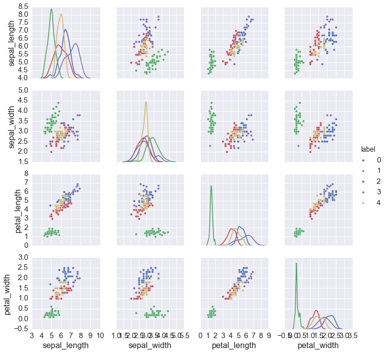
In [20]:
labels, best = best_fit(iris.ix[:, :4], 1, 11, 'aic')
iris['label'] = labels
sns.pairplot(iris, hue='label', diag_kind='kde',
            x_vars=iris.columns[:4], y_vars=iris.columns[:4])
pass
Using BIC
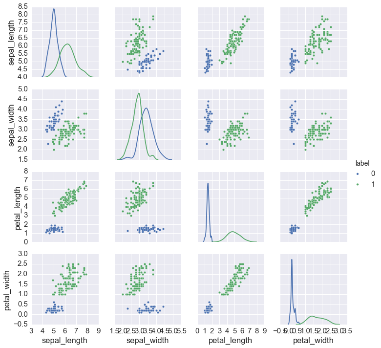
In [21]:
labels, best = best_fit(iris.ix[:,:4], 1, 11, 'bic')
iris['label'] = labels
sns.pairplot(iris, hue='label', diag_kind='kde',
            x_vars=iris.columns[:4], y_vars=iris.columns[:4])
pass
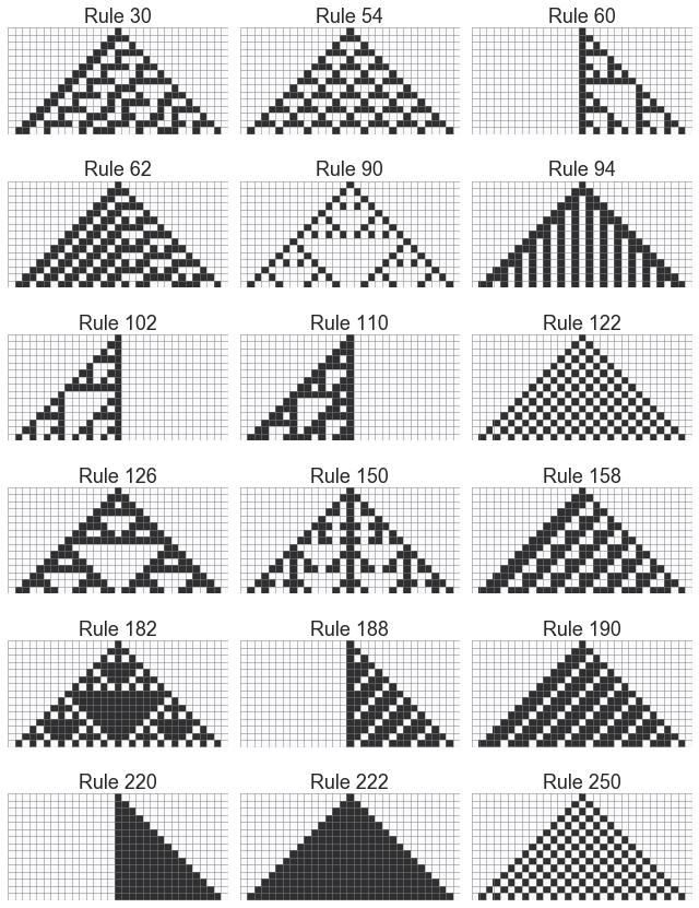
Q5. (50 pts)
Write code to generate a plot similar to the following  using
the explanation for generation of 1D Cellular Automata found
here.
You should only need to use standard Python,
using
the explanation for generation of 1D Cellular Automata found
here.
You should only need to use standard Python, numpy and
matplotllib.
In [22]:
def make_map(rule):
    """Convert an integer into a rule mapping nbr states to new state."""
    bits = map(int, list(bin(rule)[2:].zfill(8)))
    return dict(zip(range(7, -1, -1), bits))
In [23]:
def make_ca(rule, init, niters):
    """Run a 1d CA from init state for niters for given rule."""
    mapper = make_map(rule)
    grid = np.zeros((niters, len(init)), 'int')
    grid[0] = init
    old = np.r_[init[-1:], init, init[0:1]]
    for i in range(1, niters):
        nbrs = zip(old[0:], old[1:], old[2:])
        cells = (int(''.join(map(str, nbr)), base=2) for nbr in nbrs)
        new = np.array([mapper[cell] for cell in cells])
        grid[i] = new
        old = np.r_[new[-1:], new, new[0:1]]
    return grid
In [24]:
from matplotlib.ticker import NullFormatter, IndexLocator

def plot_grid(rule, grid, ax=None):
    if ax is None:
        ax = plt.subplot(111)
    with plt.style.context('seaborn-white'):
        ax.grid(True, which='major', color='grey', linewidth=0.5)
        ax.imshow(grid, interpolation='none', cmap='Greys', aspect=1, alpha=0.8)
        ax.xaxis.set_major_locator(IndexLocator(1, 0))
        ax.yaxis.set_major_locator(IndexLocator(1, 0))
        ax.xaxis.set_major_formatter( NullFormatter() )
        ax.yaxis.set_major_formatter( NullFormatter() )
        ax.set_title('Rule %d' % rule)
In [25]:
niter = 15
width = niter*2+1
init = np.zeros(width, 'int')
init[width//2] = 1
rules = np.array([30, 54, 60, 62, 90, 94, 102, 110, 122, 126,
                  150, 158, 182, 188, 190, 220, 222, 250]).reshape((-1, 3))

nrows, ncols = rules.shape
fig, axes = plt.subplots(nrows, ncols, figsize=(ncols*3, nrows*2))
for i in range(nrows):
    for j in range(ncols):
        grid = make_ca(rules[i, j], init, niter)
        plot_grid(rules[i, j], grid, ax=axes[i,j])
plt.tight_layout()
In [ ]: