TensorFlow and Edward

Packages

• TensorFlow

• TFLearn

• Keras

• Edward

References

• A Tour of TensorFlow

• Data Flow Graphs Intro

• Edward: A library for probabilistic modeling, inference, and criticism

• Deep Probabilistic Programming

TensorFlow

• A Python/C++/Go framework for compiling and executing mathematical expressions

• First released by Google in 2015

• Based on Data Flow Graphs

• Widely used to implement Deep Neural Networks (DNN)

• Edward uses TensorFlow to implement a Probabilistic Programming Language (PPL)

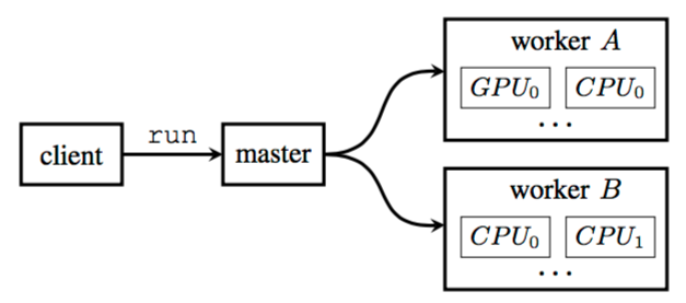
• Can distribute computation to multiple computers, each of which potentially has multiple CPU, GPU or TPU devices.

Data flow graph

• Operations

• Tensors

• Constants, variables, placeholders

• Sessions

DFG

Execution model

Agents

• Client

• Master

• Workers

• Devices

Agents

Placement algorithm

• Kernel on device?

• Size of input and output tensors

• Expected execution time

• Heuristic for cross-device transmission time

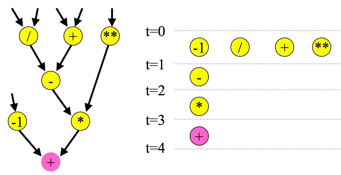
Optimization 1: Common subgraph elimination

Before	After

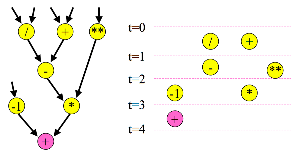
Optimization 2: As late as possible (ALAP) scheduling

ASAP	ALAP

• Lossy compression for cross-device transmission

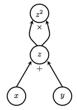
Automatic differentiation

• Symbol-to-symbol calculation of gradient

• Used for back-propagation in neural networks

• Used for gradient based optimization, HMC etc in Edward

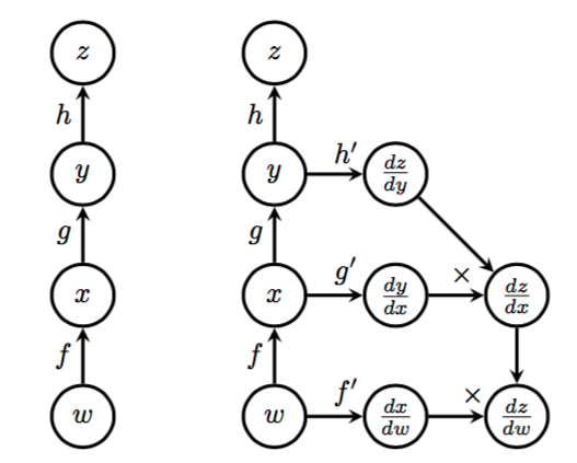
Chain rule

Other features

• Control flow (if and while) - enable recursion and cycles

• Checkpoints

  • save

  • restore

• TensorBoard visualization

  • Graphs

  • Scalar summaries (e.g. evaluation metrics)

  • Histogram summaries (e.g. weight distribution)

Abstraction layers

• Deep Neural Networks

  • contrib.learn

  • tflearn

  • tf-slim

  • keras

• Probabilistic Programming Language

  • edward

TensorFlow Examples

Hello world

import tensorflow as tf

h = tf.constant('Hello')
w = tf.constant(' world!')
hw = h + w

with tf.Session() as s:
    ans = s.run(hw)

hw

<tf.Tensor 'add:0' shape=() dtype=string>

ans

b'Hello world!'

Arithmetic on data flow graphs

a = tf.constant(5)
b = tf.constant(2)
c = tf.constant(3)
d = tf.multiply(a, b)
e = tf.add(b, c)
f = tf.subtract(d, e)

with tf.Session() as s:
    fetches = [a, b, c, d, e, f]
    ans = s.run(fetches)

ans

[5, 2, 3, 10, 5, 5]

Using operators

a = tf.constant(5)
b = tf.constant(2)
c = tf.constant(3)
d = a * b
e = b + c
f = d - e

with tf.Session() as s:
    fetrches = [a,b,c,d,e,f]
    ans = s.run(fetches)

ans

[5, 2, 3, 10, 5, 5]

Placeholders

import numpy as np

x_data = np.random.randn(5, 10)
w_data = np.random.randn(10, 1)

x = tf.placeholder('float32', (5, 10))
w = tf.placeholder('float32', (10, 1))
b = tf.fill((5,1), -1.0)

xwb = tf.matmul(x, w) + b
v = tf.reduce_max(xwb)

with tf.Session() as s:
    ans = s.run(v, feed_dict={x: x_data, w: w_data})

ans

9.055994

Linear regreession

n, p = 1000, 3

α = -1.0
β = np.reshape([0.5, 0.2, 1.0], (3,1))
x_data = np.random.randn(n, p)
y = α + x_data @ β + np.random.randn(n, 1)

x = tf.placeholder('float32', [None, p])
y_true = tf.placeholder('float32', [None, 1])

a = tf.Variable(0.0, dtype='float32')
b = tf.Variable(np.zeros((3,1), dtype='float32'))

y_pred = a + tf.matmul(x, b)

ϵ = 0.5
loss = tf.reduce_mean(tf.square(y_true - y_pred))
optimizer = tf.train.GradientDescentOptimizer(learning_rate=ϵ)
train = optimizer.minimize(loss)
init = tf.global_variables_initializer()

steps = 5
with tf.Session() as session:
    session.run(init)

    for i in range(1, steps):

        session.run(train, feed_dict={y_true: y, x: x_data})

        if i% 1 == 0:
            a_, b_ = session.run([a, b])
            print('iter={}'.format(i))
            print('a = {}'.format(a_))
            print('b = {}'.format(b_.ravel()))
            print()

iter=1
a = -0.9617397785186768
b = [ 0.58339775  0.21545935  0.97747314]

iter=2
a = -0.9741984009742737
b = [ 0.57611543  0.22001249  1.00742912]

iter=3
a = -0.9753177762031555
b = [ 0.57605499  0.2206755   1.00737011]

iter=4
a = -0.9753146171569824
b = [ 0.57600915  0.22066851  1.00741804]

MNIST digits classificaiton (canonical toy example)

Collection of \(28 \times 28\) pixel images of hand-written digits. Objective is to classify image into one of ten possile classes. State of the art DNN methods can achieve accuracy of approxmately 99.8% accuracy.

Digits

1. Download the data using input_data from tutorials.mnist

2. Declare x, W, y_true and y_pred

3. Define loss function

4. Define minimization algorithm

5. Define evaluation metrics

6. Start a session to

   1. Run loop for minimization of batches

   2. Run evaluation metric on test data

from tensorflow.examples.tutorials.mnist import input_data

n, p = 784, 10
steps = 1000
batch_size = 100
alpha = 0.5

data_dir = '/tmp/data'

data = input_data.read_data_sets(data_dir, one_hot=True)

x = tf.placeholder(tf.float32, [None, n])
W = tf.Variable(tf.zeros([n, p]))

y_true = tf.placeholder(tf.float32, [None, 10])
y_pred = tf.matmul(x, W)

loss = tf.reduce_mean(
    tf.nn.softmax_cross_entropy_with_logits(logits=y_pred, labels=y_true))

gd = tf.train.GradientDescentOptimizer(alpha).minimize(loss)

correct_mask = tf.equal(tf.arg_max(y_pred, 1), tf.arg_max(y_true, 1))
accuracy = tf.reduce_mean(tf.cast(correct_mask, tf.float32))

with tf.Session() as s:
    s.run(tf.global_variables_initializer())

    # train
    for i in range(steps):
        batch_xs, batch_ys = data.train.next_batch(batch_size)
        s.run(gd, feed_dict={x: batch_xs, y_true: batch_ys})

    # test
    ans = s.run(accuracy, feed_dict={x: data.test.images, y_true: data.test.labels})

ans

0.91790003

Using the tflearn abstraction layer

This just implements logistic regresion. Note that we can get much better perofrmance using DNN, but that is not covered here.

! pip install --quiet tflearn

import tflearn
import tflearn.datasets.mnist as mnist

X, Y, validX, validY = mnist.load_data(one_hot=True)

# Building our neural network
input_layer = tflearn.input_data(shape=[None, 784])
output_layer = tflearn.fully_connected(input_layer, 10, activation='softmax')

# Optimization
sgd = tflearn.SGD(learning_rate=0.5)
net = tflearn.regression(output_layer, optimizer=sgd)

# Training
model = tflearn.DNN(net, tensorboard_verbose=3)
model.fit(X, Y, validation_set=(validX, validY), n_epoch=3)

Training Step: 2579  | total loss: 0.25304 | time: 28.264s
| SGD | epoch: 003 | loss: 0.25304 -- iter: 54976/55000
Training Step: 2580  | total loss: 0.24640 | time: 29.406s
| SGD | epoch: 003 | loss: 0.24640 | val_loss: 0.28411 -- iter: 55000/55000
--

model.evaluate(validX, validY)

[0.92030000000000001]

Edward

Overview

• Named after George Edward Pelham Box

Model

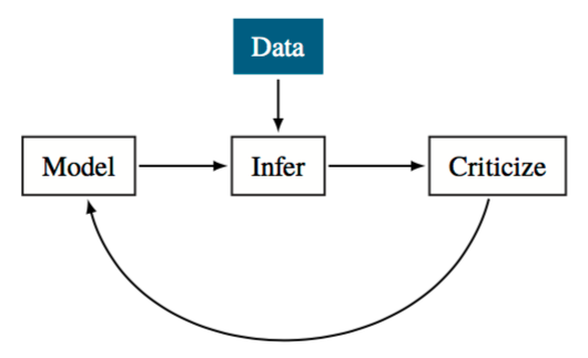
Data

• numpy arrays or tensorflow tensors

• tnesorflow placeholders

• tensorflow data readers

Model

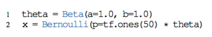
• A model is a joint distribution \(p(x, z)\) of data \(x\) and latent variables \(z\)

• A random variable has a distribution parametrized by a parameter tensor \(\theta^*\)

• Each random variable is associated to a tenor

  \[x^* \sim p(x \mid \theta^*)\]

• Random variables can be combined with other TensorFlow operations

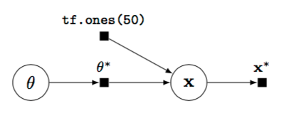
Models are built by composing random variables

Beta-Bernoulli Model | :————————-:| | | |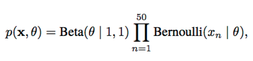

Types of models

• Directed graphical models

• Neural networks

• Bayesian non-parametric models

• Probabilistic programs (stochastic control flow with contingent dependencies)

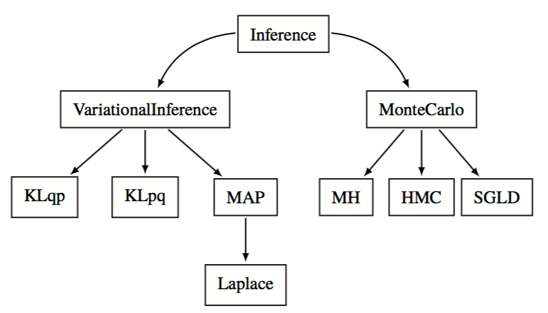
Inference

• Posterior inference

  \[q(z, \beta; \lambda) \approx p(z, \beta | x)\]

• Parameter estimation

  \[\text{optimize} \; \hat{\theta} \leftarrow p(x; \theta)\]

• Conditional inference

  \[q(\beta)q(z) \approx p(z, \beta \mid x)\]

Methods for inference

• Variational inference

  • MAP is a special case with point mass RVs

• Monte Carlo

• Composition of inference

  • Hybrid algorithms (e.g. EM variants)

  • Message passing algorithms (e.g. expectation propagation)

Methods

Criticize

Point-based evaluations

• Evaluation metrics

  • Classification error

  • Mean absolute error

  • Log-likelihood

Posterior predictive checks (PPC)

• Posterior predictive distribution

  \[p(x_\text{new} \mid x) = \int{p(x_\text{new} \mid z) p(z \mid x) dz}\]

• Procedure

  • Draw sample from posterior predictive distribution

  • Calculate test statistic on sample (e.g. mean, max)

  • Repeat to get distribution of statistic

  • Compare test statistic on original data to distribution

Edward examples

Linear Regreessiion

import edward as ed
from edward.models import Normal

Data

n, p = 1000, 3

α = -1.0
β = np.reshape([0.5, 0.2, 1.0], (3,1))

# data for training
x_train = np.random.randn(n, p)
y_train = α + x_train @ β + np.random.normal(0, 1, (n,1))
y_train = y_train.ravel()

# data for testing
x_test =  np.random.randn(n, p)
y_test = α + x_test @ β + np.random.normal(0, 1, (n,1))
y_test= y_test.ravel()

Model

Given data \((x, y)\),

\[\begin{split}p(w) = \mathcal{N}(w, 0, 1) \\ p(b) = \mathcal{N}(b, 0, 1) \\ p(y \mid w, b, x) = \prod_{i=1}^{n} \mathcal{N}(y_i \mid x_i^T w + b, 1)\end{split}\]

Note that we label the intercept \(\alpha\) as the bias \(b\) and the coefficeints \(\beta\) as weights \(w\) following neural network conventions.

X = tf.placeholder(tf.float32, [n, p])
w = Normal(mu=tf.zeros(p), sigma=tf.ones(p))
b = Normal(mu=tf.zeros(1), sigma=tf.ones(1))
y = Normal(mu=ed.dot(X, w) + b, sigma=tf.ones(n))

Inference

We fit a fully factroized variational model by minimizing the Kullback-Leibler divergence.

qw = Normal(mu=tf.Variable(tf.random_normal([p])),
            sigma=tf.nn.softplus(tf.Variable(tf.random_normal([p]))))
qb = Normal(mu=tf.Variable(tf.random_normal([1])),
            sigma=tf.nn.softplus(tf.Variable(tf.random_normal([1]))))

inference = ed.KLqp({w: qw, b: qb}, data={X: x_train, y: y_train})
inference.run()

1000/1000 [100%] ██████████████████████████████ Elapsed: 7s | Loss: 1438.422

Criticism

Find the posterior predictive distrbution.

y_post = ed.copy(y, {w: qw, b: qb})
# This is equivalent to
# y_post = Normal(mu=ed.dot(X, qw) + qb, sigma=tf.ones(N))

Calculate evalution metrics.

print("Mean squared error on test data:")
print(ed.evaluate('mean_squared_error', data={X: x_test, y_post: y_test}))

print("Mean absolute error on test data:")
print(ed.evaluate('mean_absolute_error', data={X: x_test, y_post: y_test}))

Mean squared error on test data:
1.03445
Mean absolute error on test data:
0.813144

Check parameters (true, prior, posterior)

list(zip(β, w.eval(), qw.eval()))

[(array([ 0.5]), -0.39793062, 0.52038413),
 (array([ 0.2]), 0.39972538, 0.15367131),
 (array([ 1.]), -0.095560297, 0.97044563)]

 α, b.eval(), qb.eval()

(-1.0, array([-0.54414594], dtype=float32), array([-0.9823342], dtype=float32))

More examples

See tutorials