import os
import sys
import glob
import matplotlib.pyplot as plt
import numpy as np
import pandas as pd
%matplotlib inline
%precision 4
np.random.seed(1)
plt.style.use('ggplot')
import scipy.stats as st
Computational problems in statistics
Starting with some data (which may come from an experiment or a simulation), we often use statsitics to answer a few typcical questions:
- How well does the data match some assumed (null) distribution [hypotehsis testing]?
- If it doesn’t match well but we think it is likely to belong to a known family of distributions, can we estiamte the parameters [point estimate]?
- How accurate are the parameter estimates [interval estimates]?
- Can we estimate the entire distribution [function estimation or approximation]?
Most commonly, the computational approaches used to address these questions will involve
- minimization off residuals (e.g. least squeares)
- Numerical optimization
- maximum likelihood
- Numerical optimization
- Expectation maximization (EM)
- Monte Carlo methods
- Simulation of null distribution (bootstrap, permutation)
- Estimation of posterior density (Monte Carlo integration, MCMC, EM)
Rarely (i.e. textbook examples), we can find a closed form solution to these problems.
Textbook example - is coin fair?
Data comes from simulation.
n = 100
pcoin = 0.62 # actual value of p for coin
results = st.bernoulli(pcoin).rvs(n)
h = sum(results)
print h
62
# Expected distribution for fair coin
p = 0.5
rv = st.binom(n, p)
mu = rv.mean()
sd = rv.std()
mu, sd
(50.0000, 5.0000)
Using z-test approximation with continuity correction
Use of approximation when true solution is computatioanlly expensive.
z = (h-0.5-mu)/sd
z
2.3000
2*(1 - st.norm.cdf(z))
0.0214
Using simulation to estimate null distribution
Use simulaiton when we don’t have any theory (e.g. data doesen’t meet assumptions of test)
nsamples = 100000
xs = np.random.binomial(n, p, nsamples)
2*np.sum(xs >= h)/(xs.size + 0.0)
0.0202
Maximum likelihood estimate of pcoin
Point estimate of parameter.
print "Maximum likelihood", np.sum(results)/float(len(results))
Maximum likelihood 0.62
Using bootstrap to esitmate confidenc intervals for pcoin
Interval etsimate of parameter.
bs_samples = np.random.choice(results, (nsamples, len(results)), replace=True)
bs_ps = np.mean(bs_samples, axis=1)
bs_ps.sort()
print "Bootstrap CI: (%.4f, %.4f)" % (bs_ps[int(0.025*nsamples)], bs_ps[int(0.975*nsamples)])
Bootstrap CI: (0.5200, 0.7100)
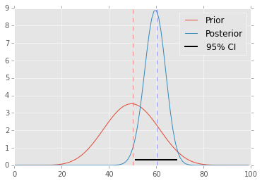
Bayesian approach
The Bayesian approach directly estimates the posterior distribution, from which all other point/interval statistics can be estimated.
a, b = 10, 10
prior = st.beta(a, b)
post = st.beta(h+a, n-h+b)
ci = post.interval(0.95)
map_ =(h+a-1.0)/(n+a+b-2.0)

xs = np.linspace(0, 1, 100)
plt.plot(prior.pdf(xs), label='Prior')
plt.plot(post.pdf(xs), label='Posterior')
plt.axvline(mu, c='red', linestyle='dashed', alpha=0.4)
plt.xlim([0, 100])
plt.axhline(0.3, ci[0], ci[1], c='black', linewidth=2, label='95% CI');
plt.axvline(n*map_, c='blue', linestyle='dashed', alpha=0.4)
plt.legend();
Comment
All the above calculations have simple analytic solutions. For most real life problems reuqireing more complex statistical models, we will need to search for solutions using more advanced numerical methods and simulations. However, the types of problems that we will be addressing are largely similar to those asked of the toy coin toss problem. These include
- point estimation (e.g. summary statistics)
- interval estimation (e.g. confidence intervals or Bayesian credible intervals)
- function estimation (e.g. density estimation, posteriro distributions)
and most will require some knowledge of numerical methods for
- optimization (e.g. least squares minimizaiton, maximum likelihood)
- Monte Carlo simulations (e.g. Monte Carlo integration, MCMC, bootstrap, permutation-resampling)
The next section of the course will focus on the ideas behiind these numerical methods.