WWWFinanceTM
Global Financial Management
Capital Structure and Dividend Policy
Copyright 1997 by Campbell R. Harvey and Stephen Gray.
All rights reserved. No part of this lecture may be reproduced without
the permission of the authors.
Latest Revision: January 4, 1997
10.0 Objectives:
After completing this class, you should be able to:
- Compute the firm's Weighted Average Cost of Capital (WACC) when there
are no taxes and when there are corporate taxes.
- Compute the required return demanded by equity-holders when there are
no taxes and when there are corporate taxes.
- Evaluate investment decisions where the project is financed in a different
proportion of debt and equity than is the existing firm and has a different
risk.
- Lever and unlever betas to reflect differences in capital structures.
- Compute appropriate required returns for projects in industries different
from the existing assets of the firm.
10.1 Introduction
In this class we address the question of how a firm should raise funds
to finance its investments. There are two alternative classes of the source
of funds.
Equity funds can be raised by issuing shares to shareholders who then
have an ownership interest in the firm. Debt funds can be raised by borrowing
from a bank or by issuing bonds. The lenders or bondholders have a creditor
relationship with the firm. The firm's financing decision is whether to
raise all funds by equity issues; to use only debt issues; or, to use a
combination of the two. Under standard economic assumptions the combination
of debt and equity chosen by a firm does not affect the market value of
the firm. That is the debt/equity decision is irrelevant to the value of
the firm. This is the famous Modigliani and Miller irrelevance proposition,
one of the cornerstones of modern finance.
When standard economic assumptions are relaxed to include corporate
taxes, and in particular deductibility of interest expenses for tax purposes,
then a levered firm (one with debt) will always be worth more than an unlevered
firm. When personal taxes are admitted in addition to corporate taxes there
are a wide range of circumstances under which the tax advantage of debt
disappears and we can arrive back at the Modigliani and Miller irrelevance
proposition.
Since the notation becomes quite extensive when examining these issues,
we begin with a reference table that defines the various symbols used in
the analysis. The terms in the table are defined throughout the text. In
general, the superscript denotes whether the symbol applies to a levered
or an unlevered firm and the subscript refers to whether the symbol applies
to (1) stocks or bonds, or (2) the existing assets of the firm or the new
project under consideration, and so on.
| Symbol |
Unlevered Firm
|
Levered Firm
|
| Value of Firm |
VU
|
VL
|
| Value of Shares (Equity) |
EU
|
EL
|
| Value of Bonds (Debt) |
-
|
DL
|
| Required Return on Shares |
reU
|
reL
|
| Required Return on Bonds |
-
|
rd
|
| Perpetual Coupon Payment |
-
|
C
|
| Average Cost of Capital |
r*U = reU
|
r*L
|
| Corporate Tax Rate |
t
|
t
|
| Risk of Existing Assets |
ßaU
|
ßaL
|
| Risk of New Project |
ßpU
|
ßpL
|
| Required Return of Existing Assets |
raU
|
raU
|
| Required Return of New Project |
rpU
|
rpU
|
10.2 Dividends: An Introduction
There are many reasons for paying dividends and there are many reasons
for not paying any dividends. As a result, dividend policy is controversial.
The term dividend usually refers to a cash distribution of earnings.
If it comes from other sources, it is called a liquidating dividend.
It mainly has the following types:
- Regular dividends are those the company expects to maintain, paid quarterly
(sometimes monthly, semiannually or annually).
- Extra dividends are those that may not be repeated.
- Special dividends are those that are unlikely to be repeated.
- Stock dividends are paid in shares of stocks. Similar to stock splits,
both increase the number of shares outstanding and reduce the stock price.
10.3 How Do Firms View Dividend Policy
In a classic study, Lintner surveyed a number of managers in the 1950's
and asked how they set their dividend policy. Most of the respondents said
that there was a target proportion of earnings that determined their policy.
One firm's policy might be to pay out 40% of earnings as dividends whereas
another company might have a target of 50%. This would suggest that dividends
change with earnings. Empirically, dividends are slow to adjust to changes
in earnings. Lintner suggested an empirical model whereby changes in dividends
are linked to the level of the earnings, the target payout and the adjustment
rate. He asserts that more "conservative" companies would be
slower to adjust to the target payout if earnings increased. The following,
from Brealey and Myers, details his research.
| 10.4 Dividend Policy
Suppose that a firm always stuck to a target payout ratio. Then the
dividend payment in the coming year (DIV1) would equal a constant
proportion of earnings per share (EPS1).
DIV1 = target dividend = (target ratio) EPS1
The dividend change would equal
DIV1 - DIV0 = (target change) = (target
ratio) EPS1 - DIV0
A firm that always stuck to its payout ratio would have to change its
dividend whenever earnings changed. But the managers in Lintner's survey
were reluctant to do this. They believed that shareholders prefer a steady
progression in dividends. Therefore, even if circumstances appeared to
warrant a large increase in their company's dividend, they would move only
partway toward their target payment. Their dividend changes therefore seemed
to conform to the following model:
DIV1 - DIV0 = (adjustment rate) (target
change) =
(adjustment
rate) (target ratio x EPS1 - DIV0)
The more conservative the company, the more slowly it would move toward
its target and, therefore, the lower would be its adjustment rate.
|
Current Year
Direction of Change
|
PreviousYear
Direction of Change
|
TwoYear
Direction of Change
|
Companies Increasing Dividend
|
Companies Maintaining Dividend
|
Companies Decreasing Dividend
|
|
+
|
+
|
+
|
81%
|
8%
|
11%
|
|
+
|
+
|
-
|
67
|
15
|
18
|
|
+
|
-
|
+
|
58
|
17
|
25
|
|
-
|
+
|
+
|
54
|
15
|
32
|
|
+
|
-
|
-
|
49
|
18
|
34
|
|
-
|
+
|
-
|
45
|
19
|
36
|
|
-
|
-
|
+
|
35
|
17
|
48
|
|
-
|
-
|
-
|
25
|
25
|
50
|
|
10.5 MM Dividend Irrelevancy without Personal
Taxes
Under the assumptions of homogeneous expectations and perfect market,
the Miller and Modigliani (MM) dividend irrelevancy proposition asserts:
While dividends are relevant, the dividend policy is irrelevant.
This proposition is perhaps best understood by studying two examples:
| Example 10.6
Suppose a firm, with 100 shares of stocks, has cash flows of $100 in
perpetuity. Assume the discount rate is 10%. Consider the following dividend
policies of the company:
1. Pay $1 dividend each year.
The stock price should be

2. Pay $2 dividend next period and pay the remainder afterwards
To pay a $2 dividend, the company has to issue a debt of $100 next year.
As a result, it also obliged to make interest payments of $10 = 10% x $100
in perpetuity starting from year 2. This implies that it has only $90 leftover
for dividends, or $.90 per share. So, the price will be:
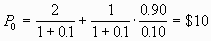
which is the same price.
3. Pay each shareholder 1 share of stock today
The firm then has 200 shares of stocks outstanding today. Since each
entitles only $.50 dividend, it must sell at

However, each original owner now has two shares of stock, his or her
wealth is
2 P0 = $10
so it will remain unchanged.
|
| Example 10.7
Suppose an all-equity firm has $2,000 cash flow residual (cash flow
minus net investment). If the firm's value, including the $2,000 residual,
is $42,000 and has 1,000 shares of stocks outstanding, consider two dividend
policies of the firm:
1. Pay $2 dividend Ex-dividend
The price is $40,000/1,000 = $40, so shareholder's wealth is $42.
2. Pay $3 dividend and raise $1,000 in new equity
Ex-dividend price is ($39,000 / 1,000) = $39;
Number of new shares is ($1,000 / 39) = 25.64;
Ex-dividend price after new equity-financing is ($40,000 / $1025.64) =
$39
So the shareholder's wealth is:
$39 + $3 = $42
and remains unchanged.
|
10.8 Summary of Factors That Could Affect Dividend
Policy
Given that the firm's investment policy is fixed, MM show that the dividend
policy is irrelevant. However, if capital market imperfections (e.g., taxes)
are important or if dividend announcements signal new information, dividend
policy will be relevant. In fact, there are important factors in dividend
policy decision that are against high dividend payout and factors are in
favor of high dividend payout and those that may affect dividend payout
either way. A list of them is:
Factors Against High Dividend Payout
- Personal Taxes. (Dividends are taxed, but capital gains are deferred;
The latter tax rate used to be lower; Since Tax Reform Act of 1986, equal
treatment.)
- Transaction Costs (From reinvesting and firm's financing.)
Factors Favoring High Dividend Payout
- Tax Reasons (80% dividend exclusion rule; institutional investors)
- Legal and Institutional Reasons (e.g., Prudent man rule)
- Desire for Current Income
- Other Factors
- The Clientele Effect
Information Content of Dividends
Other than paying dividends, a company has alternatives
- Select Additional Capital Budgeting Projects
- Share Repurchase
- Acquire Other Companies
- Purchase Financial Assets
10.9 Explanation of Factors
Personal Taxes
Before the Tax Reform Act of 1986, dividends and capital gains
were taxed at different rates. Under the old laws, dividends were taxed
as ordinary income (tax rate Tdiv of 50%) but you were
only taxed on 40% of the capital gains (Tcapgain tax
rate of 20%).
Under the old system, it seemed like individuals should prefer capital
gains because
Tcapgain < Tdiv.
Second, you are not taxed on the capital gain until it is realized.
So you can defer your taxation.
Under the Tax Reform Act of 1986 dividends and capital gains
are treated symmetrically. Beginning in the 1988 tax year, the rate of
taxation on both dividends and capital gains is a maximum of 28%. With
the new legislation, it is more difficult to make the argument that corporations
should not pay dividends because investors prefer capital gains, although
the tax deferrment of capital gains still affects dividend payout.
One should also note that there are many large institutional investors
that are tax exempt -- like pension funds. For these institutions, it is
not even possible to tell a story about tax deferral. The institutions
should be indifferent between a high dividend paying stock and a low dividend
paying stock.
The only way to determine whether there is a tax effect makes dividend
policy relevant is to empirically examine the data to see which group dominates
the data. For example, Black and Scholes (1974) formed portfolios of stocks
based on dividend payout ratios. Each of these portfolios was adjusted
for risk with the Capital Asset Pricing Model. Black and Scholes wanted
to see if there was any significant difference in total rates of return
across portfolios that was related to dividend policy. There results showed
that there was no significant difference. This implies that the market
does not reward any particular dividend policy.
The bottom line on the tax issue depends on who the marginal investor
is in the market. If the marginal investors are large tax exempt institutions
(which is likely to be the case), then they will eliminate any tax effect.
If one stock is somehow rewarded for a particular dividend policy, the
pension funds will buy in and drive the price up until that particular
firm is no different from any other firm in the same risk class.
10.10 Transaction Costs
First, the investor must incur the transactions costs of reinvesting
the dividend income. Second, the firm may have to pay for floatation costs
(if dividend is financed by new equity) or some fees for borrowing.
10.11 Tax Reasons
The main item here is the fact that a large pool of investors are institutions
which are tax-exempt. If this is not the case, such as when a large portion
of a company is still held by the family of the founder, then dividend
policy may be adjusted to maximize their after tax wealth.
10.12 The Clientele Effect
There are groups of individuals with different preferences for how they
get the cash flows from the firm. Some shareholders may prefer stocks that
do not pay dividends. Other shareholders may prefer stocks that pay a regular
dividend. Although we have seen how people can construct their own dividend
policy, there are some that "prefer" -- for whatever reason --
a certain type of dividend policy.
Investors will form their well-diversified portfolios of stocks to have
the desired dividend policy. In equilibrium, no firm can affect its value
by changing its dividend policy. If a firm did change the policy, it would
be dropped by one clientele and picked up by another. Clearly, one clientele
is as good as another. All clienteles would prefer not to be constantly
rebalancing their portfolios as firm switch policies. Rebalancing is expensive
due to transactions costs. Hence, all investors transactions costs are
minimized if the firm maintains a stable dividend policy.
10.13 Information Content of Dividends
There may be information content to dividends. The dividend may be a
signal to the public of the management's anticipations for future policy
of the firm and prospects. If there is new good information, then managers
may signal this information to the public by raising dividends. There is
a reluctance to lower dividends because managers want the dividends to
represent expectations of the future value of the firm.
An obvious question is why don't the managers inform the public about
new prospects by press releases or other non-dividend related methods?
In fact, the managers do make use of the press to announce new prospects.
The problem is credibility. Why should the public believe them? Furthermore,
there is an obvious bias because it is unlikely that they will phone a
reporter to tell them bad news. The dividend is a more credible means of
conveying information because it is costly to the firm. The more costly
the signal the more believable it is.
10.14 Capital Structure: An Introduction
There are many methods for the firm to raise its required funds. But
the most basic and important instruments are stocks or bonds. The firm's
mix of different securities is known as its capital structure. A natural
question arises: What is the optimal debt-equity ratio? For example, if
you need $100 million for a project, should all this money be raised by
issuing stocks, or 50% of stocks and 50% of bonds (debt-equity ratio equals
1), or some other ratios?
Modigliani and Miller (MM) showed that the financing decision doesn't
matter in perfect capital markets. Their famous Proposition I states
that the total value of a firm is the same with whatever debt-equity ratio
(assuming no taxes). If this is true, the basic exercise in capital budgeting
(in Bond Valuation) can be directly applied to project evaluation for firms
with different debt-equity ratios. Remember that we have implicitly assumed
firms are all-equity financed in previous lectures. However, in practice,
capital structure does matter. Then why do we bother to learn the MM's
theory? This theory is valid under certain conditions. If the theory is
far from true, so are the conditions. An understanding of the MM's theory
helps us to understand those conditions, which, in turn, helps us to understand
why a particular capital structure is better than another. In addition,
the theory tells us what kinds of market imperfection we need to look for
and pay attention to. The imperfections that are most likely to make a
difference are taxes, the costs of bankruptcy and the costs of writing
and enforcing complicated debt contracts.
10.15 MM Proposition I and Proposition II: No
Tax Scenario
MM Proposition I concerns the irrelevancy of capital structure
to the value of the firm. Notice that in what follows financial instruments
are assumed to take only two forms: stocks and bonds. In this set up, the
value of a firm is defined as:
VL = EL + DL
where DL is the market value of the levered firm's
debt and EL is the market value of the levered firm's
equity.
| 10.16 Examples
Suppose a firm has $10 million debt and 5 million shares of stock. Assume
the stock sells at a market price of $20, then
VL = 10,000,000 + 5,000,000 (20) = $110,000,000
Suppose a firm earns $100 in perpetuity. It is all-equity with 100 shares
of stock. If each sells for $10, the value
VU = 100 ($10) = $1,000
Now assume the CEO suddenly decided the firm should issue $500 dollars
of debt. The equilibrium price of the stock will drop to $5 per share and
so the value of the levered firm:
VL = 500 + (100 x 5) = $1,000
the same as before.
Why should the stock price drop to $5 per share? To understand it, suppose
you own one share of the stock.
Case 1. Unlevered:
Assume the firm pays $1 dividends in perpetuity and the interest rate
is 10%. You are willing to pay $10 for the stock because
P0 = $1.00 / 0.1 = $10.00
Case 2. Levered:
After leverage, the firm has to pay interest, $50 =500 x 10%, on the
$500 debt each period. So it can only pay $0.50 dividends in perpetuity.
As a result, the price for the stock is
P0 = $0.50 / 0.1 = $10.00
Assume the debt money was distributed to you today from the CEO, that
is $5 per share, then you still have in total $10. So, for you, as a shareholder,
you don't care what capital structure the firm has.
|
To obtain MM Proposition I, we make assumptions:
- Homogeneous expectations
- Homogeneous business risk
- Perpetual cash flows
- Perfect capital market
- Perfect competition (every one is a price taker)
- Firms and investors can borrow and lend at the same rate
- Equal access to all relevant information
No transaction cost (taxes or bankruptcy costs)
10.17 MM Proposition I
The value of the levered firm, VL, must be equal to
the value of the unlevered firm, VU.
The firm's market value and average cost of capital are completely independent
of the capital structure that the firm chooses. That is:
VL = VU
where
- VU is the value of an unlevered or all equity firm
- VLis the value of a levered firm (a firm which has
some debt in its capital structure).
Click here for
the proof
10.18 MM Proposition II
As an investor, you are concerned about the expected return on your
money, so you ask: what happens to the stock's expected return under different
debt-equity ratios?
To answer the above question, let us define r*L
as the cost of capital to a levered firm, or the overall required rate
of return:
r*L = (Expected earnings to be
paid to investors) / (Value of the firm)
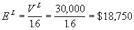
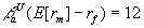
| Example 10.19
If Intel is expected to earn $1 billion next year and its value is $12
billion.
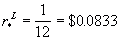
|
Now let
- DL = the market value of the firm's debt
- EL = the market value of the firm's equity
- rd = the interest rate, or return on debt
- re = the expected return on equity, or the cost of
equity
Then the expected earnings to be paid to all investors:
Expected earnings = (Earnings to bondholders) + (Earnings to
Shareholders) = rdDL + reEL
Dividing DL + EL on both sides we
get:
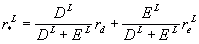
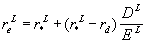
Solving for reL we have the MM Proposition
II.
The expected return on equity is a linear function of the debt-equity
ratio in the form:

Notice that, by MM Proposition I, r* stays
constant with different capital structures. In particular, it represents
the expected return when the company is all-equity financed. Since the
expected return on risky assets is generally greater than the riskless
rate, we know r*L > rd
is generally true as well. Thus, MM Proposition II implies that,
in general, the higher the debt-equity ratio, the higher the expected return
on equity.
The expected rate of return on the stock or equity of a levered firm
(reL) equals the average cost of capital plus
a risk premium equal to the debt-equity ratio times the spread between
r*L and rd that is,
Click here for
the proof
10.20 MM -- Graphical Representation
In a world with no corporate taxes, the MM Propositions can be represented
graphically as follows:

| Example 10.21
Two firms (L and U) are the same in all respects except
capital structure. Firm L has a total market value of $15,000, a
debt-equity ratio of one, and an interest rate on its perpetual bonds of
seven percent. Firm U has a total market value of $11,000 and is
unlevered. The income before interest is $2,000 for each firm, and there
are no corporate taxes.
Can costless arbitrage profits be earned, and if so how? Be specific
about the arbitrage transactions and the amount of profit earned. In which
directions will prices move as a result of the arbitrage activity, and
when will the arbitrage activity stop?
Analysis:
We know from the Modigliani and Miller irrelevance proposition that
VU = VL
Here the levered firm has a market value of $15,000 and the unlevered
firm has a market value of $11,000, implying that costless arbitrage profits
can be earned. To capture these profits, we sell ø percent
of the levered firm's shares, sell ø percent of the levered
firms bonds, and buy ø percent of the unlevered firm's shares.
This arbitrage has the following payoffs:
| Position |
Time 0
|
Time 1
|
| Sell ø of levered firm�s stock |
7,500 ø
|
-(2,000 - 525) ø
|
| Sell ø of levered firm�s bonds |
7,500 ø
|
-525 ø
|
| Buy ø of unlevered firm�s shares |
-11,000 ø
|
2,000 ø
|
| Total |
4,000 ø
|
0
|
We note that since

that
Thus C = rd DL = 0.07 (7,500)
= $525.
Costless arbitrage profits can be earned under this arrangement, so
the market cannot be in equilibrium. In the above arbitrage transactions,
ø is a value between 0 and 1, so the amount of arbitrage
profit depends on this proportion. The arbitrage activity causes the levered
firm share price to fall and the unlevered firm share price to rise and
stops where the net investment cost in the above table equals zero or where
VL = VU.
|
10.22 MM Proposition I and Proposition II: With
Corporate Taxes
In the real world, corporations are taxed at rates as high as 34%. However,
there is a quirk in the US tax code that only those earnings after interest
payments are taxable. This is one of the most important reasons for firms
to use debt financing. To understand it, let us first re-examine our previous
Example.
| Example 10.23
Recall the example of a firm, with 100 shares of stocks, which has pretax
cash flows of $100 in perpetuity. Assume the discount rate is 10%. The
tax rate is 34%. Consider the following:
Case 1. Unlevered:
The earnings after taxes are $66, so the firm can pay only $0.66 dividends
in perpetuity.
Case 2. Levered:
After leverage, the firm has interest payments of $50 each period. It
pays taxes on the remaining $50 of income. After paying taxes, it can pay
$0.33 dividends in perpetuity. So

|
Notice that the value with leverage has increased from $660 to $830.
Where does the extra amount,
$170 = $830 - $660, come from? Intuitively, the value of the firm is a
pie. It is sliced between the owners of the firm (shareholders and bondholder,
if any) and the government. In the unlevered case, the government takes
34% away. But in the levered case, only 50% of the pie is taxable and so
the government effectively takes only 17%. The total pie is the present
value of the earnings, $1000. So the government takes 17% x $1000 = $170
less in the levered case than in the unlevered case. This amount adds to
the value that the owners of the firm can enjoy:

where the tax shield is the tax rate multiplied by the present value
of the dollar interest payments.
10.24 MM Proposition I (with corporate taxes)
The general case is that the value of the levered firm is:
and the value of the unlevered firm is computed from the formula:
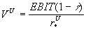
where t is the corporate tax rate; EBIT
is the expected earnings before interest and taxes; and r*U
is the discount rate for an all-equity firm (after tax).
Click here
for the proof
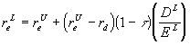
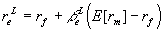
10.25 MM Proposition II (with corporate taxes)
The expected rate of return on stock of a levered firm (reL)
equals the cost of capital of an otherwise identical unlevered firm (reU)
plus a risk premium equal to the debt-equity ratio (DL
/ EL) times the spread between reU
and rd times one minus the tax rate, that is,

Click here
for the proof
10.26 MM with Taxes -- Graphical Representation
In summary, in a world with corporate taxes, the MM Propositions can
be represented graphically as follows:

| Example 10.27
Two firms L and U are the same in all respects except
capital structure. Firm L has a total market value of $30,000, a
debt-equity ratio of 0.6, and an interest rate on its perpetual bonds of
six percent. Firm U has a total market value of $26,000 and is unlevered.
The income before interest is $4,000 for each firm, and the corporate tax
rate is forty percent. Can costless arbitrage profits be earned, and if
so how? Be specific about the arbitrage transactions and the amount of
profit earned. In which directions will prices move as a result of the
arbitrage activity and when will the arbitrage activity stop?
Analysis:
The levered firm has a market value of $30,000 and a debt-equity ratio
of 0.6.
Now D L / E L = 0.6 implies that
0.6 D L = E L and since
V L = D L + E L
we have
V L = E L+0 .6 E L
or
Hence D L = V L - E L
= $11,250.
The coupon payment C is given by C = rdD
L = 0.06 (11,250) = 675.
We know from Modigliani and Miller (with corporate taxes) that
V L = V U +
t D L
If the corporate tax rate is 40 percent, then
30,000 < 26,000 + .4 (11,250) = 30,500
so the levered firm is undervalued or the unlevered firm is overvalued
or both. To capture the arbitrage profits, we sell a proportion of the
unlevered firm's shares, buy a (1-t) proportion
of the levered firm's bonds, and buy a proportion of the levered firm's
shares. This arbitrage has the following payoffs:
| Position |
Time 0
|
Time 1
|
| Sell ø of unlevered firm�s stock |
26,000 ø
|
ø 4,000 (1-0.4)
|
| Buy ø (1-t) of levered firm�s
bonds |
-ø (1.0 - 0.4) 1,250
|
ø (1-0.4) 675
|
| Buy ø of levered firm�s stock |
-ø 1,875
|
ø (4,000-675) (1-0.4)
|
| Total |
500 ø
|
0
|
Costless arbitrage profits can be earned under this arrangement, so
the market cannot be in equilibrium. At the prices reported in the question,
costless arbitrage profits of 500ø may be earned. The arbitrage
activity causes the unlevered firm share price to fall and the levered
firm share price to rise and stops where the net investment cost in the
above table equals zero or where V L = V U
+ t D L.
|
10.28 Modigliani and Miller With Corporate and Personal
Taxes
The previous section established that the introduction of corporate
taxes gives rise to a real advantage in issuing debt. In fact, a levered
firm will always be worth more than an otherwise identical unlevered firm
in the presence of corporate taxes. In this section we consider personal
as well as corporate taxes.
In Miller's famous Debt and Taxes paper, he finds that there
are a wide range of combinations of tax rates (personal and corporate)
such that the tax advantage of debt disappears. For example, consider the
case where the proceeds from stock are taxed differently to the proceeds
from corporate bonds (interest income) at the personal level. In fact if
the personal tax rate on the proceeds of stock is very small (or zero)
and the personal tax rate on interest equals the corporate tax rate the
gains from leverage will disappear. We will thus arrive back to the original
Modigliani Miller irrelevance proposition -- the debt/equity decision is
irrelevant to the value of the firm.
10.29 Ivestment Evaluation and Capital Structure
In this section, we consider how the capital structure issues introduced
above impact upon investment decisions. In particular, we examine how to
compute the required return for a particular investment under the assumptions
that MM Proposition I with corporate taxes holds and that the firm
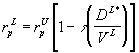
has decided its target capital structure, DL* / VL.
In a world where corporate taxes exist, the required rate of return
on a risky project is given by
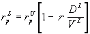
where rpU is the required rate of return
on an unlevered firm in the same risk class as the project in question.
That is, we calculate the return required for the risk involved in the
project rpU (given by the CAPM) and then adjust
this rate for taxes. In this sense, rpU is
a pure required return which reflects only the risk of the project. It
is not affected by tax considerations because there are no tax-deductible
interest payments in the unlevered firm. This is consistent with the way
we compute Net Present Values (NPVs). When we calculate the incremental
cash flows of the project we do so on an after tax basis. It is only sensible
therefore to calculate the NPV using an after tax required rate of return.
Click here
for the proof
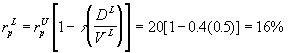
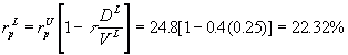
| 10.20 Example (Capital Structure Change):
A company currently has a market value of $4 million, 25 percent of
which is bonds. Its average cost of capital is 18 percent, and its corporate
tax rate is 40 percent. The company is evaluating a $800,000 investment
project which is expected to generate after-tax cash flows of $176,000
a year indefinitely. The project is in the same risk class as the existing
assets of the firm. If the project is accepted, it will be financed such
that the post-investment debt ratio is 0.5. The riskless rate of interest
is 8%. Should the project be accepted?
Analysis:
We note that the required rate of return for the project in this levered
firm (rpL)given by
where rpU is the required return on an
identical project in an unlevered firm. Plugging in the unknowns here we
have
18 = rpL [1 - 0.4 (0.25)]
which implies that
rpU = 20%.
Now with the capital structure change we calculate our new required
rate of return using
DL* / VL = 0.5
Thus the NPV is given by
NPV = 176,000 / 0.16 - 800,000 = $300,000
and therefore we would accept the project.
|
| 10.31 Example (Risk Change):
A company currently has a market value of $4 million, 25 percent of
which is bonds. Its average cost of capital is 18 percent, and its corporate
tax rate is 40 percent.. The company is evaluating a $800,000 investment
project which is expected to generate after-tax cash flows of $176,000
a year indefinitely. The project is 40 percent riskier than the firm's
average operations. The riskless rate of interest is 8 percent. Should
the project be accepted?
Analysis:
Because the new project is not in the same risk class as the existing
assets of the firm, we subscript returns and betas with p
if they relate to the new project and a if they relate to the existing
assets of the firm. We note that the required rate of return of the current
assets of the levered firm raL is given by
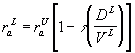
Plugging in the unknowns here we have
18 = raU [1 - 0.4 (0.25)]
which implies that
raU = 20%
Now raU is the required return on an all
equity firm in the same risk class as our existing levered firm and hence
raU is given by the CAPM:
which implies that
Now the beta of our project (ßpU)
is 40% higher than the beta of the existing assets (ßaU)
thus

and hence

Plugging this back into the formula for required return we find
Thus
NPV= 176,000 / 0.2232 - 800,000= -$11,469.53
and therefore we reject the project.
|
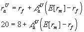
| 10.32 Example (Risk Change/Capital Structure
Change):
A company currently has a market value of $4 million, 25 percent of
which is bonds. Its average cost of capital is 18 percent, and its corporate
tax rate is 40 percent. The company is evaluating a $800,000 investment
project which is expected to generate after-tax cash flows of $176,000
a year indefinitely. The project is 40 percent riskier than the firm's
average operations, and, if it is accepted, it will be financed such that
the post-investment debt ratio is 0.5. The riskless rate of interest is
8 percent. Should the project be accepted?
Analysis:
Once again, a p subscript denotes the project being investigated
and an a subscript denotes the existing assets of the firm. We note that
the required rate of return of the current assets of this levered firm
raL is given by
Plugging in the unknowns here we have
18 = raU [1 - 0.4 (0.25)]
which implies that
raU = 20%.
Now raU is the required return on an all
equity firm in the same risk class as our levered firm and hence raU
is given by the CAPM:
which implies that
Now the beta of our project (ßpU)
is 40% higher than the beta of the existing assets (ßaU)
thus
and hence
When we plug this back into the formula for required return we also
note that the new value of
DL / VL = 0.5
and hence:
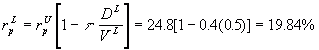
and
NPV = 176,000 / 0.1984 - 800,000 = $87,096.77
we therefore accept the project.
|
10.33 Computing an Appropriate
Discount Rate
In this section we seek to evaluate a new investment opportunity for
the firm where the appropriate discount rate is unknown. We would be able
to compute this discount rate directly from the CAPM if the appropriate
beta for the new project was known, however in this section we consider
the case where the beta of the new project is unknown. Often, however,
we will be able to identify another company that deals primarily in the
industry from which the new project is drawn. It is a simple matter to
use historical series of (1) market returns and (2) returns from the shares
of that company to compute the beta of the shares or equity of the
company. This can be done via a simple OLS regression.
This equity beta is a measure of the risk of holding shares in
the particular company and comprises two risks. First, there is an inherent
business or asset risk from holding the particular type of assets owned
by the firm. For example, the airline industry is inherently riskier than
the soda manufacturing industry, so the assets of United Airlines
would have a higher beta than the assets of Coca-Cola. Second,
there is leverage risk stemming from the company having debt in its capital
structure. This reflects the fact that equity holders have a residual claim
on the assets of the firm. In the event of bankruptcy, the debtholders
must be paid out in full before the equityholders receive any payment.
Moreover, consider a new firm that wants to buy a single asset that
costs $100 and will either generate a profit of $10 or a loss of $5 over
the first period. If the firm finances this investment with ten $10 shares,
each share will either be worth either $11 or $9.50 at the end of the period.
If, however, the firm borrows $50 and issues only five shares, each share
will be worth either $12 [(100+10-50)/5] or $9 [(100-5-50)/5]. Clearly,
shares in the levered firm are riskier in the sense that the distribution
of possible outcomes is more diverse. Since the equityholders face higher
risk, they will demand a higher required return. However this simple example
ignores the tax benefits from issuing debt. That is, the firm will have
to pay interest to the debtholders, but these interest payments are tax
deductible. That is, there are two effects:
- The leverage effect: The equityholders face higher risk due to the
fact that there are debtholders with a prior claim over the firms assets.
This tends to increase the beta and required return on equity.
- The tax subsidy effect: The interest payments to the debtholders are
subsidized by the government by way of tax deductibility. This tends to
lessen the return demanded by equityholders and hence decreases the equity
beta.
The strategy for computing the appropriate beta to use in evaluating
the project is to first determine the beta of a related company�s
equity. Then unlever that beta (remove the effects of leverage and
tax subsidies) leaving just a beta that reflects the pure business
risk of that type of asset. Finally re-lever this pure beta to incorporate
the leverage and tax subsidy effects applicable to our firm, and use the
CAPM to find the appropriate required return for the project.
10.34 Unlevering Equity Betas
This section demonstrates how to remove the effects of leverage (having
debt in the capital structure) from the beta of equity in a levered firm
(ßeL) leaving a beta that reflects the
pure business risk of the assets (ßeU).
From Modigliani and Miller Proposition 2 (with corporate taxes)
we have
Substitute in from the CAPM
and
and we find that
where ßeU is the beta of shares
of an unlevered firm and ßeL is the
beta of shares of a levered firm with
debt/equity ratio of DL / EL.
| Example 10.35
A firm has a market value of $100 million, 20% of which is bonds. The
company is considering a $10 million investment project that is expected
to earn after-tax cash flows of $3 million per year for the next 8 years.
The beta of the firm's shares is 1.0. The expected return on the
market is 12% and the T-Bill rate is 4%. The corporate tax rate is 40%.
This project is 20% riskier than the firm's average operations. If the
project is accepted, the post-investment debt ratio will be 0.4. Should
the project be accepted?
Step 1:
The decision rule for determining whether any project should be accepted
or rejected is based on NPV. The first step is always to check what information
is required to calculate the NPV. This will involve two components: a series
of cash flows and an appropriate discount rate. In this case, we know the
cash flows, but the appropriate discount rate is one which incorporates
(1) the risk of this kind of project, and (2) the effect
of the tax deductibility of debt in this levered firm. We call this discount
rate rpL and note that it is not yet known.
We can, therefore, express the NPV of the project as:
Step 2:
From step 1, we are missing a discount rate and there are two
obvious places to look. The CAPM is specifically designed to tell us what
discount rate to use if we know the appropriate beta, ßpL:

Alternatively, if we know the discount rate appropriate for this type
of project in an unlevered firm, we can make an adjustment for the tax
deductibility of debt:
Step 3:
If we decide to use the CAPM in step 2, we need to compute ßpL.
This can be done by adjusting some other ß (which we know)
for differences in risk and capital structure. In this case, we know that
the beta of the firm's equity with the current capital structure, ßeL*,
is 1.0, where L* denotes that the current capital structure is different
from the post-investment capital structure if the project is accepted.
The first thing we can do is remove the effects of the tax deductibility
of debt, leaving us with a beta that reflects only the risk of the
current assets of the firm. That is, we want to unlever this beta:
where
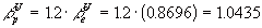
Since we have an unlevered company beta of 1, our levered beta
is 0.8696
Step 4:
We know that the risk of the project is 20% greater than the risk of
the existing assets of the firm, so
Step 5:
At this point, note that we can find the required return on our project
in an unlevered firm from the CAPM:

Step 6:
Now we can return to step 2 and use the second formula:

Step 7:
Finally, we can return to step 1 and compute the NPV of the project:
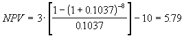
Since the NPV is positive, we would accept the project.
|
10.36 Implications of the MM Theory
The market value of a levered firm equals the market value of an unlevered
firm plus the present value of interest tax shields. In order to get the
simple expression above, we have assumed that the debt is perpetual. More
generally, the tax shield term would be the present value of the interest
tax shields.
The implication of the model with corporate taxes is that the value
of the firm is maximized when it is financed entirely by debt. This is
not a very attractive implication for the model. Clearly, no firm is financed
100% by debt. There are a number of real world constraints that need to
be considered.
- There are institutional and legal restrictions (some institutions will
not purchase stock of a firm that has a debt-equity ratio that exceeds
some cutoff).
- There are costs imposed for going bankrupt that might persuade the
firm's management not to increase the debt-equity ratio too high.
- The interest tax shield may exhaust taxable income (this suggests an
upper bound on the amount of debt). Finally, there may be conflicts of
interest between stockholders and bondholders.
Each of these points suggests that the 100% debt policy may not be optimal
for a firm. If we look to the market, the average debt to value ratio is
less than 40%. Furthermore, a survey of 768 of the largest industrial firms
shows that 126 (16%) have no debt in their capital structures. This empirical
evidence suggests that the 100% debt policy is clearly not what is observed.
The wide range of debt-equity ratios in the market could indicate that
the original proposition about the irrelevance of the capital structure
may have more merit than we initially gave it.
10.37 Bankruptcy Costs
There are many costs involved in bankruptcy. The direct costs are legal
fees and court costs. The indirect costs arise from discontinued operations,
the hesitancy of customers to purchase the product and the unwillingness
of suppliers to extend any credit. These costs make it unlikely that a
firm will push its debt-equity ratio very high. If we take the bankruptcy
costs into account, then there may be an optimal capital structure where
the marginal tax advantage equals the marginal bankruptcy costs. Note that
the marginal bankruptcy costs may be different across firms. This may explain
why all firms do not have the same level of debt-equity.
10.38 Exhausting the Benefits
Obviously, if the firm is unlikely to earn taxable profits, the effective
tax shield is small. As a result, it should not borrow.
10.39 Conflicts of Interest
Once the debt is outstanding, shareholders have the incentive to take
actions that benefit themselves at the expense of the bondholders. So if
there is debt outstanding, the objectives of maximizing the value of the
firm and the value of the equity are not identical. Some examples of bondholder-shareholder
conflicts are: claim dilution, dividend payout and asset
substitution. Let's examine in more detail some of these conflicts.
Consider claim dilution. With debt outstanding, stockholders have incentives
to issue claims of equal or senior priority. The proceeds from the "new"
debt issue will be greater the higher the priority of the new debt. The
claim dilution increases the risk of the "old" debt and its market
value falls. The combined value of the new and old debt is fixed. By making
new debt an equal or higher priority, the value of the old debt falls and
the proceeds from the new debt issue rises. Claim dilution benefits the
stockholders at the expense of the "old" bondholders.
But the bondholders are not stupid. The price of the bonds equals the
present value of the expected cash flows. The bondholders include the affects
of conflicts of interest in estimating cash flows and pricing the debt.
Bondholders only pay for what they expect to get.
Since the conflicts of interest between stockholders and bondholders
reduce the price of the debt, the stockholders bear all of the costs of
the conflict. Even though the shareholders bear the costs of the conflict,
there is still an incentive to extract value or expropriate from the bondholders
-- after the debt is outstanding.
Since the stockholders bear the costs that arise from the conflicts
of interest, they have an incentive to minimize the agency costs. Bond
covenants are detailed enforceable contracts that reduce agency costs by
restricting the stockholders' actions after the debt is issued. The covenants
may restrict the production and investment policy (e.g., mergers, sale
of certain assets and lines of business). The covenants may restrict the
financial policy of the firm (e.g., dividend payouts, priority and total
debt). Furthermore, there is usually a provision for auditing. The bond
covenants will reduce but will not eliminate these agency costs. Note that
there are also costs involved in monitoring the firm's actions.
10.40 Capital Structure as Options
I mentioned that both the debt and the equity of the firm could be considered
options. Let's explore this idea in some more detail. The bondholders are
promised payments of $A next period. If default occurs, then the
bondholders own the firm. The stockholders receive all residual cash flows
after the payments to bondholders. Consider the distribution of the value
of the firm.

Now consider the payoff schedule. Suppose the debt has time to maturity,
T. The standard deviation of the firm's value is sigma.
| Payments to: |
If V < A
|
If V > A
|
Position
|
| Stockholders |
0
|
V-A
|
Call with Strike A,
Time to maturity T
Standard Dev Sigma
|
| Bondholders |
V
|
A
|
V - Call
|
| Total |
V
|
V
|
V
|
The call option is a function of the exercise price, A, the time
to maturity, T, and the standard deviation of the return on the
underlying asset, sigma. The payments to the stockholders and bondholders
add up to the total cash flows of the firm.
Consider the position diagrams. The position diagram for the call option
is straightforward.
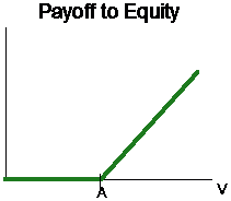
Note that V represents the value of the firm at the expiration
or final payment of the principal on the debt. This diagram indicates that
the stockholders have a call option on the value of the firm. The payoff
is determined by Max[0, V-A].
The position diagram for bondholders is slightly more complicated.
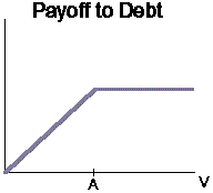
The bondholders hold the value of the firm and write a call option (the
shareholders buy it in the form of common equity). Combining the payoffs
of the long position in the value of the firm with a short position in
the call delivers the above diagram. The payoff stream is Min[V, A].
Acknowledgment
Some of the material for this lecture is drawn from Richard Ruback's
note, "Dividend Policy."