WWWFinance^TM

Global Financial Management

Option Contracts

Copyright 1997 by Campbell R. Harvey and Stephen Gray. All rights reserved. No part of this lecture may be reproduced without the permission of the authors.

Latest Revision: February 16, 1997

This class provides an overview of option contracts. As with forwards and futures, options belong to the class of securities known as derivatives since their value is derived from the value of some other security. The price of a stock option, for example, depends on the price of the underlying stock and the price of a foreign currency option depends on the price of the underlying currency. Options trade both on exchanges (where contracts are standardized) and over-the-counter (where the contract specification can be customized). The focus of this class is on

• Definitions and contract specifications of the major exchange-traded options,
• The mechanics of buying, selling, exercising, and settling option contracts,
• Option trading strategies including hedging, and
• The relationships between options, the underlying security, and riskless bonds. In particular, it is possible to form combinations of derivatives and the underlying security that are riskless, providing a means of valuing options.

5.1  Objectives:

After completing this class, you should be able to:

• Determine the possible payoffs of option contracts.
• Understand the mechanics of buying, selling, exercising, and settling option contracts.
• Determine the possible payoffs of portfolios of options, bonds, and the underlying asset.
• Examine market prices to determine whether arbitrage bounds are violated in option markets.
• Understand the directional effects of relevant variables on the value of options.
• Use standard valuation techniques to determine the price of options.

---

5.2  Definitions

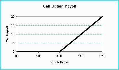
A call option is a contract giving its owner the right to buy a fixed amount of a specified underlying asset at a fixed price at any time or on or before a fixed date. For example, for an equity option, the underlying asset is the common stock. The fixed amount is 100 shares. The fixed price is called the exercise price or the strike price. The fixed date is called the expiration date. On the expiration date, the value of a call on a per share basis will be the larger of the stock price minus the exercise price or zero.

Options are in force for a limited time. The option expires when it is executed or on the expiration date (also called the maturity date). A call option on XYZ with a strike price of 45 and a maturity date in January will be referred to as "The XYZ 45 January calls." All exchange traded options in the U.S. expire on the saturday following the third friday of the expiration month.

One can think of the buyer of the option paying a premium (price) for the option to buy a specified quantity at a specified price any time prior to the maturity of the option. Consider an example. Suppose you buy an option to buy 1 Treasury bond (coupon is 8%, maturity is 20 years) at a price of $76. The option can be exercised at any time between now and September 19th. The cost of the call is assumed to be $1.50. Let's tabulate the payoffs at expiration.

Consider the payoffs diagrammatically. Notice that the payoffs are one to one after the price of the underlying security rises above the exercise price. When the security price is less than the exercice price, the option is referred to as out of the money.

A put option is a contact giving its owner the right to sell a fixed amount of a specified underlying asset at a fixed price at any time on or before a fixed date. On the expiration date, the value of the put on a per share basis will be the larger of the exercise price minus the stock price or zero.

One can think of the buyer of the put option as paying a premium (price) for the option to sell a specified quantity at a specified price any time prior to the maturity of the option. Consider an example of a put on the same Treasury bond. The exercise price is $76. You can exercise the option any time between now and September 19. Suppose that the cost of the put is $2.00.

The payoff from a put can be illustrated. Notice that the payoffs are one to one when the price of the security is less than the exercise price.

Writing or "shorting" options have the exact opposite payoffs as purchased options. The payoff table for the call option is:

Notice that the liability is potentially unlimited when you are writing options.

he put option can be similarly illustrated:

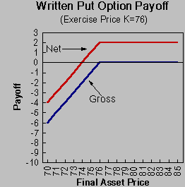
As with the written call, the upside is limited to the premium of the option (the initial price). The downside is limited to the minimum asset price - which is zero.

There are two other definitions that are needed. A European Option is an option that can only be exercised at maturity. That is, there is no opportunity for early exercise. An American Option can be exercised at any time up to the maturity date.

5.3  The Mechanics of Option Contracts

Whereas a futures contract requires settlement between the buyer and seller at maturity of the contract, an option contract is settled at the discretion of the buyer. If settlement would involve a cash flow from the seller to the buyer, the buyer will exercise his option and receive a payment from the seller. Conversely, if settlement would involve a cash flow from the buyer to the seller, the buyer will choose not to exercise the option and no funds will change hands. The buyer will only exercise the option when it is in his interest to do so, in which case the buyer will either receive a positive cash flow or nothing when the contract matures. Clearly, the buyer must offer a payment to the seller (the option premium) to induce the seller to take the other side of such a contract.

Option contracts can be classified according to whether they they give the holder the right to buy or to sell the underlying asset. A call option is a contract that gives the holder the right to buy a particular asset at a specified price (called the exercise price or strike price) within a specified period of time. A put option is a contract that gives the holder the right to sell a particular asset at a specified price within a specified period of time.

Options can be further classified according to when they may be exercised. European options may only be exercised on the expiration day, while American options may be exercised at any time up to and including the expiration day. Most options that trade on organized exchanges throughout the world are of the American kind. European options trade primarily in the over the counter market.

The following examples illustrate the mechanics of call and put options respectively.

All stock options on the CBOE (such as the IBM options in the previous examples) are of the American type. Although the above examples considered exercising at maturity, the buyer may, if he wishes, exercise at any time before maturity. An alternative way for the buyer to liquidate his option position is by issuing a sell to close order. This procedure simply involves an option buyer selling his rights under the option contract to a third party. The next example describes the process.

If the current asset price is above the strike price, the call option is said to be in the money because immediate exercise would result in a positive cash flow. Conversely, if the current asset price is below the strike price the call option is out of the money and if the current asset price equals the strike price the call option is at the money. Similarly, if the asset price is above the strike price the put option is out of the money and if the asset price is below the strike price the put option is in the money.

5.7  Claims to the Firm as Options

There are a number of situations where an option can be identified.

• Discount Corporate Bonds. Suppose that the face value of a corporate bond is $60 million and it matures in 12 months. If the firm's value at that date is less than $60 million, then the stock holders are out of the money. Hence, common stock is a call option on the value of the firm, with maturity date the date the bond matures and the exercise price is the par value of the bond.
  
• Coupon Bearing Corporate Bonds. At every time that the coupon is due, the firm faces bankruptcy. Hence, there are multiple options on the value of the firm.
  
• Convertible Bonds. This is simply a straight bond plus a call option on the stock of the firm.
  
• Callable Bonds. This is the bond minus a call on the value of the bond.
  
• Warrants. A warrant is a call issued by the firm on the firm's common equity.
  
• Executive Compensation. Often stock options are issued for executive compensation.
  
• Lease with option to buy. It is common to include in a leasing contract an option to buy the equipment.

5.8  Some Uses of Options

There are many uses for options. We will review three possible uses: writing covered calls, using options instead of stock, and obtaining portfolio insurance.

5.9  Earn Extra Money by Writing a Covered Call

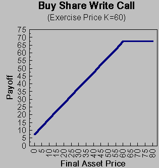
Suppose you own a share of a particular stock. You might be able to make some extra money by writing a call. Note the difference here. In this case, you are writing (not buying) the call option. Because you already own the underlying security, you are covered from infinite losses if the stock price takes off.

We can sketch the payoffs for this strategy. First, we need a few definitions. Let S^* be the ultimate value of the stock price on the maturity date. Let k be the exercise price. The call price will be denoted by c. The price of a zero coupon bond that matures on the same day as the option is denoted by B. The straight line is the payoffs from holding the stock long. The kinked solid line is the payoffs from shorting (writing) the call option. The dashed line is the net payoff. This is referred to as a hedge position. Note if the stock price stays below the exercise price, then you are clearly better off. If the stock price rises dramatically, then you do not capitalize on all the gain. The region below the dashed line denotes the gain from writing the covered call.

5.10  Using Options Instead of Stock

Suppose you have a choice of two investment strategies. The first is to invest $100 in a stock. The second strategy involves investing $90 in 6 month T-bills and $10 in 6 month calls. So we will want to buy 10/c calls. That is, if the call is priced at $5, then you are able to buy 2 calls.

The payoffs for this strategy are outlined below. Note that because we own 2 calls, the payoffs are two for one. That is for every dollar the stock price is above the exercise price, we make two dollars on the call. The diagram shows the payoffs from strategy 2. The slope of the call payoff is 2. The T-bill payout is flat. As soon as the stock price goes past the exercise price, the portfolio value rises rapidly. A comparison of the two investment strategies is outlined. Note that the option substitution strategy does not do as well if the stock price does not move that much.

5.11  Portfolio Insurance

One can obtain insurance on a portfolio of stocks by buying a put. So for every dollar that the stock portfolio drops, you make back by holding the put. So portfolio managers can cover the downside by taking out portfolio insurance. In the diagram, the solid lines represent the payoffs from the long stock position and long put position. The dashed line is the total return or the hedge position. Note that the cost of covering the downside is lower returns if the stock rises in value.

5.12  Determinants of Option Value

Now that we understand what an options contract is, we can look at how they are valued. This will be done in a few steps.

1. Options are derivative securities, which means that they derive their value from some other asset, like stock. Changing the value of that underlying stock will obviously affect the price of the option. We will evaluate the effect of stock price movements, as well as the effect of movements in other variables, such as interest rates, strike price and volatility.
   
2. Once we understand how these variables influence the option price, we will look at certain bounds on option prices which, if violated, would lead to arbitrage opportunities. Of particular importance will be the Put-Call Parity equation.
   
3. At this point, we will present the Black-Scholes model for pricing options.
   
4. After presenting the equations, we will give some intuition to these equations. While the proof of the Black-Scholes equations is beyond the scope of this class, it is important to understand some of the concepts behind these equations.

5.13  Current Stock Price

As the current stock price goes up, the higher the probability that the call will be in the money. As a result, the call price will increase. The effect will be in the opposite direction for a put. As the stock price goes up, there is a lower probability that the put will be in the money. So the put price will decrease.

5.14  Exercise Price

The higher the exercise price (or strike price), the lower the probability that the call will be in the money. So for call options that have the same maturity, the call with the price that is closest (and greater than) the current price will have the highest value. The call prices will decrease as the exercise prices increase. For the put, the effect runs in the opposite direction. A higher exercise price means that there is higher probability that the put will be in the money. So the put price increases as the exercise price increases.

Link to a Java animation showing the effect of exercise price on a call option.

5.15  Volatility

Both the call and put will increase in price as the underlying asset becomes more volatile. The buyer of the option receives full benefit of favorable outcomes but avoids the unfavorable ones (option price value has zero value).

Link to a Java animation showing the effect of volatility on a call option.

5.16  Interest Rates

The higher the interest rate, the lower the present value of the exercise price. As a result, the value of the call will increase. The opposite is true for puts. The decrease in the present value of the exercise price will adversely affect the price of the put option.

Link to a Java animation showing the effect of interest rates on a call option.

5.17  Cash Dividends

On ex-dividend dates, the stock price will fall by the amount of the dividend. So the higher the dividends, the lower the value of a call relative to the stock. This effect will work in the opposite direction for puts. As more dividends are paid out, the stock price will jump down on the ex-date which is exactly what you are looking for with a put. (There is also an issue of optimal exercise of the call and put option which will be addressed later.)

5.18  Time to Expiration

There are a number of effects involved here. Generally, both calls and puts will benefit from increased time to expiration. The reason is that there is more time for a big move in the stock price. But there are some effects that work in the opposite direction. As the time to expiration increase, the present value of the exercise price decreases. This will increase the value of the call and decrease the value of the put. Also, as the time to expiration increase, there is a greater amount of time for the stock price to be reduced by a cash dividend. This reduces the call value but increases the put value.

Link to a Java animation showing the effect of time to expiration on a call option.

5.19 Summary of Effects

Let's summarize these effects.

Determinants of Option Value
Effect of Increases

Click here to Link to Option Dynamics

---

5.20  Basic Principles of Option Valuation

Consider the following two rules:

(1) If one portfolio of securities gives a higher future payoff than another portfolio in every possible circumstance, then the first portfolio must have a higher current value than the second portfolio.

(2) If two portfolios of securities give the same future payoff in every possible circumstance, then they must have the same current value.

If (1) and (2) did not hold, then it would be possible for a professional trader to make an arbitrage profit by simultaneously selling the relatively overpriced portfolio and buying the relatively underpriced portfolio. We will use these rules to construct positions that offer the identical payoff as the option. If we can price the position with the same payoff as the option, then we have the price of the option.

Another point to note is that the modern valuation of exchange-traded options ignores margin requirements, transactions costs, and taxes because it focuses on market pricing relations that are enforced by the arbitrage activities of professional traders. The margin requirements and transactions costs of these traders are very low. Furthermore, taxes usually reduce the level of arbitrage profits but do not change the circumstances in which they occur.

5.21  Put--Call Parity (no dividends)

The price of a call and a put are linked via the put--call parity relationship. The idea here is that holding the stock and buying a put is going to deliver the exact same payoffs as buying one call and investing the present value of the exercise price. Let's demonstrate this. Consider the payoffs of two portfolios. Portfolio A contains the stock and a put. Portfolio B contains a call and an investment of the present value of the exercise price.

Since the portfolios always have the same final value, they must have the same current value. This is the rule of no arbitrage. We can express the put--call parity relation as:

Of course, this relation can be written in many different ways:

and

where PV(k) is the present value of the exercise price. Now consider a diagram for each of the payoffs.

See also Option arbitrage relations.

5.22  Put--Call Parity (with dividends)

We can also use the put-call parity theory for a stock that pays dividends. The idea is very similar to the no dividend case. The value of the call will be exactly equal to the value of a portfolio that includes the stock, a put, and borrowing the present value of the dividend and the present value of the exercise price. Consider the payoffs of two portfolios. Portfolio A just contains the call option. Portfolio B contains the stock, a put and borrowing equal to the present value of the exercise price and the present value of the dividend.

Since the portfolios always have the same final value, they must have the same current value. Again, this is the rule of no arbitrage. Note that this arrangement of the portfolios is slightly different from the case with no dividends. In the no dividends case, we had the stock and a put in portfolio A. In the dividends case, we have just the call in portfolio A. But clearly, we could have constructed the no dividends case with just a call in the portfolio A -- it would have no impact on the result. Further note, that the as result of borrowing the present value of both the dividend and the exercise price, we only payoff the exercise price. The reason for this is that if you get the dividend payment before expiration, then you use it to reduce you total debt. In fact, you use it to exactly payoff that part of the debt that is related to the dividend part of the borrowing.

We can express the put--call parity relation as:

where PV(k) is the present value of the exercise price and PV(d) is the present value of the dividend. We can be more precise about these present values:

Consider the following time line which shows the flows from buying stock at T₀:

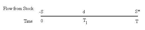
Note that we are using continuous time rates of interest here. All that is really happening is that you are selling k zero coupon bonds today. At the time of expiration, T, you have to pay those bonds off. The amount that you have to payoff is k. You are also selling d zero coupons bonds which mature at the date that the dividend is paid, T₁. For these bonds, you use the revenue from the dividend paid to pay off the bonds.

---

5.24  Arbitrage Bounds for Options

As with forward and futures markets, option markets are redundant. This is because an option on a stock is simply a means of buying or selling stock and it is already possible to buy and sell stocks in the stock market. Hence option markets are redundant and options can be valued by arbitrage. The next portion of this lecture develops a series of arbitrage bounds that must be satisfied by option prices.

5.25  American and European Options

Recall that the feature that distinguishes American options from European options is that American options can be exercised prior to expiration. Since an American option conveys all of the rights of a European option plus more (i.e., the right to exercise early) an American option must be at least as valuable as its European counterpart:

and

5.26  Lower Bound on an American Call Option

A lower bound on the value of an American call is given by:

The intuition underlying this bound is that (a) the call is a right and not an obligation to buy the stock, so it cannot have a negative value, and (b) the call may be exercised at any time up to expiration, so it must be worth at least as much as its current exercisable value S-k. The next example demonstrates how an arbitrage is possible if this bound is not satisfied.

5.28  Lower Bound on an American Put Option

Similar logic may be used to establish a lower bound for the value of an American put option:

Example 5.29 demonstrates how to execute the arbitrage in this case if the lower bound is not satisfied.

5.30  Lower Bound on a European Call Option

A lower bound on the value of a European call option is given by:

To see why this bound must hold, consider forming a portfolio that consists of a long position in the European call option C_E, a long position of k(1+r)^-T riskless bonds, and a short position in the stock at price S. The initial and terminal values of this portfolio are contained in Table 10.1.

If, at the expiration of the option, the stock price exceeds the exercise price, the net terminal portfolio value is 0. If, however, the stock price is below the exercise price at expiration, the net terminal portfolio value is positive. Since the portfolio is assured of achieving a nonnegative terminal value, with positive probability of a strictly positive value, it must have a positive price. That is

It must also be the case that the European call has a nonnegative price, so the complete lower price bound of the European call is

5.32  Lower Bound on a European Put Option

The lower bound on the price of a European put option is given by

To see why this bound must hold, consider forming a portfolio that consists of a long position in a European put option P_E, a long position in the stock S, and a short position of k(1+r)^-T in riskless bonds. The initial and terminal values of this strategy are contained in the following table.

If the stock price is below the exercise price when the put option expires, the net portfolio value will be zero. If, however, the stock price exceeds the exercise price at expiration, the net portfolio value will be positive. Since this portfolio provides a nonnegative terminal value and positive probability of a strictly positive value, it must have a positive price. That is,

Adding the nonnegativity constraint for the value of a European put option yields

5.35  Distribution of Returns

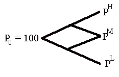
There is one very important aspect of determining the prices of options that we have said little about so far -- the distribution of outcomes. If we know how asset prices are distributed, we should be able to determine an actuarily fair value for them. For example, suppose an asset is worth $100 now. Suppose, in this idealized example, that we know that in one week the asset will either be worth $80 or it will be worth $125. Knowing that these are the only outcomes, we should be able to to compute the value of an option (say a call option with a strike price of $110)) on this asset. Let's look further into this situation.

5.36  Option Valuation in the Binomial Model

This analysis is concerned with call options only, but all concepts extend to put options. The framework is the binomial model, although all the concepts described here extend to more general models, hence the analysis has wider applications. The following notes are intended to help you in gaining a deeper understanding of the underlying concepts.

This section uses the following notation:

Consider the following binomial tree:

In this simplified world, we will price the option using three different methods:

1. The Arbitrage method. Using this method, we construct a portfolio with the same payoffs as the option. By the principal of no arbitrage free profits, this portfolio must have the same price as the option.
2. The Contingent Claims Method. Here, we are using the same method, except that the portfolio we construct is made up of contingent claims -- which pay off only in one state of the world. Note, in this example, we only have two payoff states.
3. The Risk Neutral Method. Recall that the risk averting investor is not willing to take a fair bet, because he prefers the sure thing. In a world where investors are risk neutral, assets would be priced at their fair price. This will just be the sum of the payoff in each state times the probability of that state occurring. Note that if an investor who is risk averting can eliminate his risk for free, he will take a fair bet. While options are thought of as being very risky, they can be combined with their underlying assets to eliminate certain types of risk. Thus, we might suppose that a risk averter might be willing to pay the fair price for an option.

5.37  Arbitrage

Arbitrage is based on the law of one price: two portfolios of financial claims with identical payoffs in all states must also cost the same. We have seen this method before, when we priced assets by replicating their cash flows with other assets.

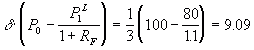
The method is therefore to construct a portfolio which always has the same payoff as the option. The principle of arbitrage is to replicate the payoffs of the option. In order to create the replicating portfolio, define:

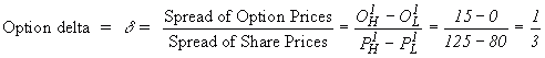
Then the portfolio which replicates the option consists of two assets (assume the option is worthless in the low state,
i. e., O₁^L = 0). Call this portfolio X.

1.  Buy delta shares of the asset.

2. Borrow (i.e., sell a bond) worth

which is the present value of delta times P₁^L

Hence, this portfolio replicates the option. By the arbitrage principle the option and this portfolio must trade at the same price, and we can conclude that the option value is O₀ = 9.09.

Valuation by arbitrage works in two steps:

1. Construct a portfolio like portfolio X with identical payoffs to the option for all states.
2. Invoke the principle of arbitrage and conclude the value of the option today equals the current value of portfolio X.

We assumed that O₁^L = 0. If the option has a value in this state, it only affects the amount that we borrow. The argument still works.

An important (and surprising) thing to note is that nowhere did we make reference to the probabilities of each state. It doesn't matter if the low state has a 10% chance of occurring or a 70% chance.

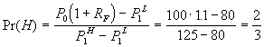
5.38  Contingent Claims Pricing

In this simplified example, Contingent Claims Pricing differs little from what we have just seen. However, in a situation where there are multiple possible payoff states, this method does differ from the Arbitrage method. The idea is that we want to find the price of an asset which pays off exactly $1 in a given state, and pays nothing in all other states. In this case, we have two different assets that we would price. The first pays $1 in the high state, and nothing in the low state. The second pays $1 in the low state and nothing in the high state.

Once we calculate these values, we can then price the option by looking at its payoffs in each state, and determining how many of the contingent claim assets we would need to replicate the option's payoffs.

From here it is easy to construct two portfolios which both pay off $1 in the high state and nothing in the low state. These two portfolios are:

1. (1 / O₁^H ) of the option (i. e. 1/15 options in the example).
2. (1 / O₁^H ) of the portfolio X (i. e. 1/15 the portfolioin the example).

By the principle of arbitrage, both portfolios cost the same, and they both pay off $1 in the high state and nothing in the low state. Hence, it is legitimate to define the state price in-dependently of the portfolio as the value of a security paying off $1 in this state. The easiest procedure to construct such a portfolio in the current case is:

1. Borrow P₁^L / (1 + R_f) = 80 / 1.1 = 72.73, and buy one share.

This portfolio pays off P₁^H-P₁^L = 45 in the high state and 0 in the low state.

2. Buy of this portfolio. The cost of this portfolio is simply:

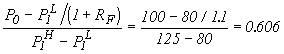
However, since any portfolio with this payoff structure costs the same by the arbitrage principle, any portfolio which pays off $1 in the high state and nothing in the low state would lead to the same conclusion. The rationale behind this procedure is also easy to see. The share price can be understood as a reward for two payments:

1. A payment of P₁^L = 80 for sure, independently of the state.

2. A bet on the high state, where the extra payoff P₁^H - P₁^L = 45 is only received in the high state.

Investors pay P₀ for the stock as a whole, and P₁^L / (1 + R_f) for a safe payment of P₁^L. Hence, the difference of

is a payment for the bet investors buy on top of the safe payment of P₁^L. Now, if investors pay for a bet which pays off P₁^H - P₁^L = 45 in the high state, then the state price for the high state (denoted by ) is simply:

This is the same conclusion as before: investors pay $0.606 today for $1 in the high state at the end of the period. Since an option with a zero payoff in the low and 15 in the high state is simply a portfolio with O₁^H = 15 times this payoff, the value of the call option can be calculated as:

Hence, the state price can be determined by decomposing the share price into a payoff for a fixed payment plus a payment for the bet on a high payoff. The option can than be val-ued by using the state price. How would this method apply if the strike price of the option were lower than the share price in the low state, such that O₁^L > 0? In this case we have to determine the state price for the low state as well. This is of course the price today of a security which pays off $1 in the low state and nothing in the high state, i. e. the exact re-verse of the security we looked at before. The value of this security can then be defined as the state price for the low state and denoted by . Now, a security which pays off $1 in both states is simply a riskless bond, which costs 1 / (1 + R_F). Since investing in one security which pays off $1 in the low state and nothing in the high state, and in one security which pays off $1 in the high state and nothing in the low state is the same as investing in a riskless bond with payoff $1 in both states, we can invoke the arbitrage principle and the state prices must satisfy:

The value of the share can be "derived" directly from these state prices:

Obviously, this is not a derivation since the state prices have been constructed to satisfy this equation. This gives the value of the option as:

Hence, contingent claims pricing involves two steps:

1. Infer the state prices from stock and bond prices; state prices must sum to the price of a riskless bond
    with payoff $1, stock prices can be decomposed into riskless payoffs and "bets".

2. Use the state prices to determine the value of an option. This method extends to the case were O₁^L > 0

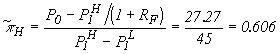
5.39  The Risk Neutral Method

Contingent claims pricing analyzes the payoff to a share as a combination of a fixed pay-ment and a bet. The risk neutral method analyzes this bet by determining the odds (or bet-ter: the probabilities) for this bet and the resulting fair price, rather than determining the state prices directly. The correctness of this method follows from the way state prices are determined. Suppose we would invest  dollars at the safe rate of interest. Then the payoff at the end of the period is:  by construction (see section on contingent claims). Similarly, investing dollars (or dollars) at the safe rate of interest pays off  (or dollars). Since these two values sum up to 1.00, by construction, they are like probabilities, and they are the probabilities needed in order to construct a fair bet. In other words, we are extracting the expected probability distribution from the state prices (contingent claims).

Hence, define the probabilities as  and . Using these probabilities, we see that the stock price is the present value of the expected value using these probabilities:

Dividing by P₀ and then subtracting 1 on both sides of the equation gives the same equation in the form of returns (this is also the equation given in Brealey and Myers on p. 575):

This equation can now be used in order to determine the probabilities of a fair bet ("risk neutral probabilities") as:

Since the same relationship holds for the option, we have

Hence, the last algorithm for pricing an option according to the "risk neutral method" is:

1. Determine the "risk-neutral" probabilities from the stock-price equation.
2. Use the same probabilities in order to determine the option value. This last method is the "risk-neutral method" described on pp. 575f. in Brealey and Myers. Whether you use the equation in terms of price levels or in terms of returns is a matter of convenience.

5.40  Binomial Model -- Comments

This note has discussed three different methods for valuing options in a binomial tree. Arbitrage uses the law of one price and values the option by constructing a replicating portfolio. The arbitrage principle implies that we can construct several portfolios which pay off $1 in one state and nothing in the others, and all these portfolios cost the same. Hence we can legitimately call the value of any such portfolio the state price, leading to valuing options as contingent claims where the payoff of the option in each state is valued by the state price. Determining state prices is similar to assuming that securities are "fair bets" which can be valued by inferring the implied probabilities or odds of such a bet. These "risk neutral probabilities" can then be used in order to value any other fair bet on the same states like an option. Hence, all three methods follow from each other, with arbitrage being in some sense the fundamental principle which forms the starting points, and the existence of state prices and risk neutral probabilities following as a consequence.

To extend this framework to valuing actual options requires two modifications. First, the terminal distribution of the stock price is unlikely to be a distribution of only a few values - a continuous distribution is desirable. Also required is a method for determining the appropriate discount rate to use for the present value calculation.

In a celebrated paper, Black and Scholes (1973) incorporate both of these features. They note that if percentage stock price changes are normally distributed (this is called geometric Brownian motion), the terminal distribution of the stock price (S_T) will be lognormal. For example, suppose that the price of Netscape stock is currently $75 and that percentage returns are normally distributed with a mean of 20% p.a. and standard deviation of 45% p.a. Under the Black-Scholes assumption of geometric Brownian motion the distribution of the terminal stock price is lognormal. Note that this distribution is positively skewed (unlike the normal distribution which is symmetric) and assigns zero probability to negative stock prices (consistent with the limited liability of shares).

Furthermore, Black and Scholes note that there are two ways of performing the present value calculation: (1) let the stock price drift upwards according to the expected return of the stock and then discount option payoffs by an appropriate expected return, or (2) pretend that the stock price drifts upward at the riskless rate and then discount option payoffs at the riskless rate. That is, we make two errors - we have the wrong expected return for the stock and the wrong discount rate for the option - but these errors always cancel exactly. This technique, is just the risk neutral valuation which we just looked at. It enables the option payoffs to be discounted at the risless rate of interest, obviating the need to compute a required return for the option.

Before giving up on the binomial model and jumping into the continuous lognormal distribution, let's take a look at how the binomial model could be modified to suit our needs. As mentioned, most options in the real world don't have two states. But the binomial model can be used to approximate those states, if the distribution of states is similar to a binomial distribution. Suppose that the example given above has a time horizon of one month. We know that a stock has more than two possible outcomes in a month. We could try to predict the price by taking two steps:

Note that we have two possible states after a half month, and three states after a full month. But why stop there? We could take daily steps, and have 30 or so possible states after a month. We could take shorter and shorter time periods, and eventually have a large number of possible states at the end of our time horizon. The probabilities associated with each state is determined by the probabilities of moving up or down at each step, and by the number of ways to get to each state. Not that in the tree above, there are two ways to get to the middle state, and only one way to get to the high and low states. The probability distribution that this creates is the binomial distribution.

If we want to use the tools of the Calculus, we can take the limit as the length of time between steps goes to zero. The binomial distribution will converge to the Normal distribution. This leads us, naturally, to our next section.

5.41  Review of the Normal Distribution

The normal distribution is a continuous bell-shaped probability distribution. The normal distribution is particularly convenient to use because the distribution can be completely described by two parameters -- the mean and the variance. Below is a diagram of a normal distribution and the actual U.S. stock returns. That is, this distribution is drawn with the historical mean and variance of the U.S. stock returns.

As you can see, stock returns are approximately normal. The Black-Scholes model assumes that stock prices follow a lognormal distribution. This is equivalent to saying that the instantaneous rate of returns on stocks is normal. Since the binomial distribution described above converges to the normal distribution, a binomial model should find the same price for an option as the Black-Scholes model.

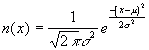
We will work with the "standard" normal. This distribution is called standard because the mean is assumed to be zero and the standard deviation is one. The area under the normal curve represents the probability. In all the options pricing examples we will be interested in cumulative probability. The interpretation is: what is the probability that the value is less than some number, x. This simply means that we are going to be summing up the area under the curve -- working from the left.

Let's consider an example. If I am given the number zero, what is the cumulative probability. Stated differently, what is the probability that the number that I draw from the distribution has the value of negative infinity to zero. What I want is the area under the curve to the left of zero. Since the curve is symmetric and since the area under the curve must sum to one, the probability is .50. If I am given the number -3, what is the probability? Viewing the diagram of the normal distribution, the -3 is way out on the left tail. The area from -3 to the left is very small (a guess would be .01). If we were given the point 3, this is way out on the right tail. The area to the left of 3 is almost the entire area under the curve (a guess would be .99).

In order to use the Black-Scholes formula, we will need precise numbers for these probabilities. We usually use a computer or a statistical table to get these probabilities.

5.43  The Black-Scholes Pricing Formula for Call Options

First, some definitions are needed.

• S = current stock (underlying asset) price
  
• k = exercise price of the option
  
• T = time to maturity of the option in years (e.g. 5 months is .408)
  
• B = price of a zero coupon (riskless) bond that pays $1.00 at maturity. This can be represented as e^{-rT}.
  
• c = call option value
  
• PV(d) = present value of the dividends to be paid to the stock prior to maturity
  
• 'sigma' = annual standard deviation of the rate of return on the stock
  
  
• N(x)= cumulative normal probability of value less than x

5.44  The Black-Scholes Formula:

There are many ways of writing the Black-Scholes formula. All of them are equivalent to the above. For example, Sharpe's text presents the formula differently. However, with some algebra, the formula is identical to the Black and Scholes formula above.

Now to get used to using the formula, it is best to do some examples. I have created a Java program which can be used to value options using the Black and Scholes formula. However, everyone should be able to code the formula into an Excel spreadsheet..

Note: many text books use the symbols d₁ and d₂ rather than x₁ and x₂.

But before we work some examples, I will try to given some of the intuition behind the formula.

5.45  Some Intuition Behind the Black-Scholes Formula

Usually, in Finance, we refer to people as risk averse. I defined this earlier as the preference for $50 for sure rather than taking a 50-50 bet with payoffs of $0 and $100. Now let's suppose that agents are risk neutral. This means that they are indifferent between the $50 for sure and the bet. If this is the case, then the value of the call can be thought of as the expected payoff of the call at expiration discounted back to present value. We could write:

Substituting the expression for present value:

Note that S^* is the stock price at expiration. This expression says that the call price is the present value of the expected expiration price minus the exercise price times the probability the call is in the money.

In terms of the Black-Scholes formula, N(x₂) can be interpreted as the probability that the call option will be in the money at expiration. The term N(x₁) is the present value of the expected terminal stock price conditional upon the call option being in the money at expiration times the probability that the call will be in the money at expiration. Finally, the term

is the present value of the cost of exercising the option at expiration times the probability that the call will be in the money at expiration. So the Black-Scholes formula for call option has a fairly simple interpretation. The call price is simply the discounted expected value of the cash flows at expiration.

5.46  Using the Black-Scholes Formula

An Options Pricer which uses the Black-Scholes model is now available.

5.48  Option Delta and Elasticity -- Call options

The option delta measures the change in the option price for a unit change in the stock price.

The delta is also known as the hedge ratio. This means that the delta tells how many shares I need to buy to hedge the sale of one call.

The Options Pricer returns the delta.For the two month call, the value is 0.59682. For the five month call, the delta is 0.59319.

The delta is just the partial derivative of the call price, taken with respect to the price of the underlying asset. That is:

The elasticity or omega is interpreted as the call option's elasticity to changes in the underlying asset's price. So if the stock price rises by 1% the call price should rise by 'omega'%. This value is also returned by the Option Pricer. We can now see the link between the delta and the omega.

5.49  Option Delta and Elasticity -- Put options

The delta of a call option is the first derivative of the Black-Scholes call formula with respect to the stock price:

The delta of a put option is the first derivative of the put formula with respect to the stock price. From put-call parity, we know:

The delta of the put is:

Simplifying,

The omega of the call option is

Similarly, the omega of the put option is

5.50  Hedging with Options

When hedging with forward or futures contracts there is no initial investment required. Forward and futures prices are set so that the contract is a fair bet in the sense that there is a 50/50 chance of being left bet ter or worse off. If the spot price were to move one way, the hedger's physical position will increase in value and the futures position will generate an offsetting loss. Conversely, if the spot price were to move the other way, the hedger's physical position will decrease in value and the futures position will generate an offsetting gain. The forward or futures hedge effectively locks in a price when the contract is entered into. The hedger gives up the gains that would accrue if the spot price were to move in one direction in order to insure against the losses that would accrue if the spot price were to move in the other direction.

An alternative way of hedging the risk that prices will move adversely is with options. In this case, a premium is paid at the time of entering the hedge in order to insure against bad outcomes. The upside potential (should prices happen to move favorably) is retained. That is, options, futures, and forwards can all be used to eliminate the risk of prices moving adversely. For futures and forwards, the price of this insurance is that the hedger gives up any upside potential. For options, the hedger retains this upside potential and instead pays an insurance fee (the option premium) at the time of entering the hedge. The following example illustrates how foreign exchange risk can be hedged using currency options.

Acknowledgement

Much of the materials for this lecture are from George Constantinides, "Financial Instruments'', John C. Cox, "Option Markets'' and Douglas Breeden, "Options.''