
ACF and PACF
plots
AR and MA signatures
A model for the UNITS series--ARIMA(2,1,0)
Mean versus constant
Alternative model for the UNITS series--ARIMA(0,2,1)
Which model should we choose?
Mixed models
Unit roots
ACF and PACF plots: After a time series has been stationarized by differencing, the next step in fitting an ARIMA model is to determine whether AR or MA terms are needed to correct any autocorrelation that remains in the differenced series. Of course, with software like Statgraphics, you could just try some different combinations of terms and see what works best. But there is a more systematic way to do this. By looking at the autocorrelation function (ACF) and partial autocorrelation (PACF) plots of the differenced series, you can tentatively identify the numbers of AR and/or MA terms that are needed. You are already familiar with the ACF plot: it is merely a bar chart of the coefficients of correlation between a time series and lags of itself. The PACF plot is a plot of the partial correlation coefficients between the series and lags of itself.
In general, the "partial" correlation between two variables is the amount of correlation between them which is not explained by their mutual correlations with a specified set of other variables. For example, if we are regressing a variable Y on other variables X1, X2, and X3, the partial correlation between Y and X3 is the amount of correlation between Y and X3 that is not explained by their common correlations with X1 and X2. This partial correlation can be computed as the square root of the reduction in variance that is achieved by adding X3 to the regression of Y on X1 and X2.
A partial autocorrelation is the amount of correlation between a variable and a lag of itself that is not explained by correlations at all lower-order-lags. The autocorrelation of a time series Y at lag 1 is the coefficient of correlation between Y(t) and Y(t-1), which is presumably also the correlation between Y(t-1) and Y(t-2). But if Y(t) is correlated with Y(t-1), and Y(t-1) is equally correlated with Y(t-2), then we should also expect to find correlation between Y(t) and Y(t-2). (In fact, the amount of correlation we should expect at lag 2 is precisely the square of the lag-1 correlation.) Thus, the correlation at lag 1 "propagates" to lag 2 and presumably to higher-order lags. The partial autocorrelation at lag 2 is therefore the difference between the actual correlation at lag 2 and the expected correlation due to the propagation of correlation at lag 1.
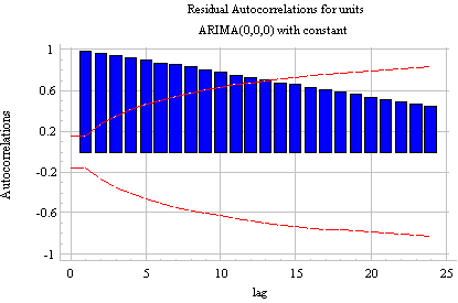
Here is the autocorrelation function (ACF) of the UNITS series, before any differencing is performed:

The autocorrelations are significant for a large number of lags--but perhaps the autocorrelations at lags 2 and above are merely due to the propagation of the autocorrelation at lag 1. This is confirmed by the PACF plot:
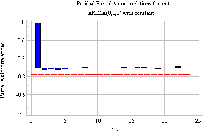
Note that the PACF plot has a significant spike only at lag 1, meaning that all the higher-order autocorrelations are effectively explained by the lag-1 autocorrelation.
The partial autocorrelations at all lags can be computed by fitting a succession of autoregressive models with increasing numbers of lags. In particular, the partial autocorrelation at lag k is equal to the estimated AR(k) coefficient in an autoregressive model with k terms--i.e., a multiple regression model in which Y is regressed on LAG(Y,1), LAG(Y,2), etc., up to LAG(Y,k). Thus, by mere inspection of the PACF you can determine how many AR terms you need to use to explain the autocorrelation pattern in a time series: if the partial autocorrelation is significant at lag k and not significant at any higher order lags--i.e., if the PACF "cuts off" at lag k--then this suggests that you should try fitting an autoregressive model of order k
The PACF of the UNITS series provides an extreme example of the cut-off phenomenon: it has a very large spike at lag 1 and no other significant spikes, indicating that in the absence of differencing an AR(1) model should be used. However, the AR(1) term in this model will turn out to be equivalent to a first difference, because the estimated AR(1) coefficient (which is the height of the PACF spike at lag 1) will be almost exactly equal to 1. Now, the forecasting equation for an AR(1) model for a series Y with no orders of differencing is:

If the AR(1) coefficient ("phi") in this equation is equal to 1, it is equivalent to predicting that the first difference of Y is constant--i.e., it is equivalent to the equation of the random walk model with growth:

The PACF of the UNITS series is telling us that, if we don't difference it, then we should fit an AR(1) model which will turn out to be equivalent to taking a first difference. In other words, it is telling us that UNITS really needs an order of differencing to be stationarized.
AR and MA signatures: If the PACF displays a sharp cutoff while the ACF decays more slowly (i.e., has significant spikes at higher lags), we say that the stationarized series displays an "AR signature," meaning that the autocorrelation pattern can be explained more easily by adding AR terms than by adding MA terms. You will probably find that an AR signature is commonly associated with positive autocorrelation at lag 1--i.e., it tends to arise in series which are slightly underdifferenced. The reason for this is that an AR term can act like a "partial difference" in the forecasting equation. For example, in an AR(1) model, the AR term acts like a first difference if the autoregressive coefficient is equal to 1, it does nothing if the autoregressive coefficient is zero, and it acts like a partial difference if the coefficient is between 0 and 1. So, if the series is slightly underdifferenced--i.e. if the nonstationary pattern of positive autocorrelation has not completely been eliminated, it will "ask for" a partial difference by displaying an AR signature. Hence, we have the following rule of thumb for determining when to add AR terms:
An MA signature is commonly associated with negative autocorrelation at lag 1--i.e., it tends to arise in series which are slightly overdifferenced. The reason for this is that an MA term can "partially cancel" an order of differencing in the forecasting equation. To see this, recall that an ARIMA(0,1,1) model without constant is equivalent to a Simple Exponential Smoothing model. The forecasting equation for this model is

where the MA(1) coefficient "theta" corresponds to the quantity "1-alpha" in the SES model. If the MA(1) coefficient is equal to 1, this corresponds to an SES model with alpha=0, which is just a CONSTANT model because the forecast is never updated. This means that when the MA(1) coefficient is equal to 1, it is actually cancelling out the differencing operation that ordinarily enables the SES forecast to re-anchor itself on the last observation. On the other hand, if the moving-average coefficient is equal to 0, this model reduces to a random walk model--i.e., it leaves the differencing operation alone. So, if the MA(1) coefficient is something greater than 0, it is as if we are partially cancelling an order of differencing . If the series is already slightly overdifferenced--i.e., if negative autocorrelation has been introduced--then it will "ask for" a difference to be partly cancelled by displaying an MA signature. (A lot of arm-waving is going on here! A more rigorous explanation of this effect is found in the "Mathematics of ARIMA Models" handout.) Hence the following additional rule of thumb:
A model for the UNITS series--ARIMA(2,1,0): Previously we determined that the UNITS series needed (at least) one order of nonseasonal differencing to be stationarized. After taking one nonseasonal difference--i.e., fitting an ARIMA(0,1,0) model with constant--the ACF and PACF plots look like this:
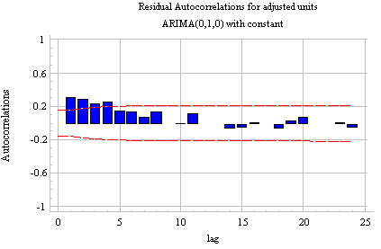
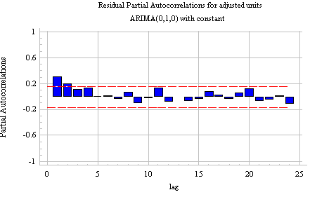
Notice that (a) the correlation at lag 1 is significant and positive, and (b) the PACF shows a sharper "cutoff" than the ACF. In particular, the PACF has only two significant spikes, while the ACF has four. Thus, according to Rule 7 above, the differenced series displays an AR(2) signature. If we therefore set the order of the AR term to 2--i.e., fit an ARIMA(2,1,0) model--we obtain the following ACF and PACF plots for the residuals:


The autocorrelation at the crucial lags--namely lags 1 and 2--has been eliminated, and there is no discernible pattern in higher-order lags. The time series plot of the residuals shows a slightly worrisome tendency to wander away from the mean:
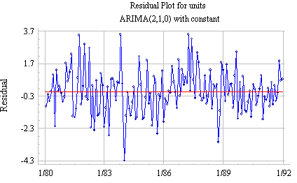
However, the analysis summary report shows that the model nonetheless performs quite well in the validation period, both AR coefficients are significantly different from zero, and the standard deviation of the residuals has been reduced from 1.54371 to 1.4215 (nearly 10%) by the addition of the AR terms. Furthermore, there is no sign of a "unit root" because the sum of the AR coefficients (0.252254+0.195572) is not close to 1. (Unit roots are discussed on more detail below.) On the whole, this appears to be a good model.
Analysis Summary
Data variable: units
Number of observations = 150
Start index = 1/80
Sampling interval = 1.0 month(s)
Length of seasonality = 12

Forecast Summary
----------------
Nonseasonal differencing of order: 1
Forecast model selected: ARIMA(2,1,0) with constant
Number of forecasts generated: 24
Number of periods withheld for validation: 30

            Estimation      Validation
Statistic   Period          Period
--------------------------------------------
MSE         2.10757         0.757818
MAE         1.11389         0.726546
MAPE        0.500834        0.280088
ME          0.0197748       -0.200813
MPE         0.0046833       -0.0778831

                            ARIMA Model Summary
Parameter           Estimate        Stnd. Error     t               P-value
----------------------------------------------------------------------------
AR(1)               0.252254        0.0915209       2.75624         0.006593
AR(2)               0.195572        0.0916343       2.13426         0.034492
Mean                0.467566        0.240178        1.94675         0.053485
Constant            0.258178
----------------------------------------------------------------------------
Backforecasting: yes
Estimated white noise variance = 2.10875 with 146 degrees of freedom
Estimated white noise standard deviation = 1.45215
Number of iterations: 1
The (untransformed) forecasts for the model show a linear upward trend projected into the future:
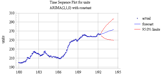
The trend in the long-term forecasts is due to fact that the model includes one nonseasonal difference and a constant term: this model is basically a random walk with growth (NF#1) fine-tuned by the addition of two autoregressive terms--i.e., two lags of the differenced series. The slope of the long-term forecasts (i.e., the average increase from one period to another) is equal to the mean term in the model summary (0.467566). The forecasting equation is:

where "mu" is the constant term in the model summary (0.258178), "phi-1" is the AR(1) coefficient (0.25224) and "phi-2" is the AR(2) coefficient (0.195572).
Mean versus constant: In general, the "mean" term in the output of an ARIMA model refers to the mean of the differenced series (i.e., the average trend if the order of differencing is equal to 1), whereas the "constant" is the constant term that appears on the right-hand-side of the forecasting equation. The mean and constant terms are related by the equation:
CONSTANT = MEAN*(1 minus the sum of the AR coefficients).
In this case, we have 0.258178 = 0.467566*(1 - 0.25224 - 0.195572)
Alternative model for the UNITS series--ARIMA(0,2,1): Recall that when we began to analyze the UNITS series, we were not entirely sure of the correct order of differencing to use. One order of nonseasonal differencing yielded the lowest standard deviation (and a pattern of mild positive autocorrelation), while two orders of nonseasonal differencing yielded a more stationary-looking time series plot (but with rather strong negative autocorrelation). Here are both the ACF and PACF of the series with two nonseasonal differences:
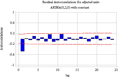
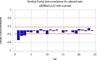
The single negative spike at lag 1 in the ACF is an MA(1) signature, according to Rule 8 above. Thus, if we were to use 2 nonseasonal differences, we would also want to include an MA(1) term, yielding an ARIMA(0,2,1) model. According to Rule 5, we would also want to suppress the constant term. Here, then, are the results of fitting an ARIMA(0,2,1) model without constant:
Analysis SummaryNotice that the estimated white noise standard deviation (RMSE) is only very slightly higher for this model than the previous one (1.46301 here versus 1.45215 previously). The forecasting equation for this model is:
Data variable: units
Number of observations = 150
Start index = 1/80
Sampling interval = 1.0 month(s)
Forecast Summary
----------------
Nonseasonal differencing of order: 2
Forecast model selected: ARIMA(0,2,1)
Number of forecasts generated: 24
Number of periods withheld for validation: 30
Estimation Validation
Statistic Period Period
--------------------------------------------
MSE 2.13793 0.856734
MAE 1.15376 0.771561
MAPE 0.518221 0.297298
ME 0.0267768 -0.038966
MPE 0.017097 -0.0148876
ARIMA Model Summary
Parameter Estimate Stnd. Error t P-value
----------------------------------------------------------------------------
MA(1) 0.75856 0.0607947 12.4774 0.000000
----------------------------------------------------------------------------
Backforecasting: yes
Estimated white noise variance = 2.1404 with 147 degrees of freedom
Estimated white noise standard deviation = 1.46301
Number of iterations: 4

where theta-1 is the MA(1) coefficients. Recall that this is similar to a Linear Exponential Smoothing model, with the MA(1) coefficient corresponding to the quantity 2*(1-alpha) in the LES model. The MA(1) coefficient of 0.76 in this model suggests that an LES model with alpha in the vicinity of 0.72 would fit about equally well. Actually, when an LES model is fitted to the same data, the optimal value of alpha turns out to be around 0.61, which is not too far off. Here is a model comparison report that shows the results of fitting the ARIMA(2,1,0) model with constant, the ARIMA(0,2,1) model without constant, and the LES model:
Model ComparisonThe three models perform nearly identically in the estimation period, and the ARIMA(2,1,0) model with constant appears slightly better than the other two in the validation period. On the basis of these statistical results alone, it would be hard to choose among the three models. However, if we plot the long-term forecasts made by the ARIMA(0,2,1) model without constant (which are essentially the same as those of the LES model), we see a significant difference from those of the earlier model:
----------------
Data variable: units
Number of observations = 150
Start index = 1/80
Sampling interval = 1.0 month(s)
Number of periods withheld for validation: 30
Models
------
(A) ARIMA(2,1,0) with constant
(B) ARIMA(0,2,1)
(C) Brown's linear exp. smoothing with alpha = 0.6067
Estimation Period
Model MSE MAE MAPE ME MPE
------------------------------------------------------------------------
(A) 2.10757 1.11389 0.500834 0.0197748 0.0046833
(B) 2.13793 1.15376 0.518221 0.0267768 0.017097
(C) 2.18056 1.14308 0.514482 0.000765696 0.0041274
Model RMSE RUNS RUNM AUTO MEAN VAR
-----------------------------------------------
(A) 1.45175 OK OK OK OK OK
(B) 1.46217 OK OK OK OK OK
(C) 1.47667 OK OK OK OK OK
Validation Period
Model MSE MAE MAPE ME MPE
------------------------------------------------------------------------
(A) 0.757818 0.726546 0.280088 -0.200813 -0.0778831
(B) 0.856734 0.771561 0.297298 -0.038966 -0.0148876
(C) 0.882234 0.796109 0.306593 -0.014557 -0.00527448
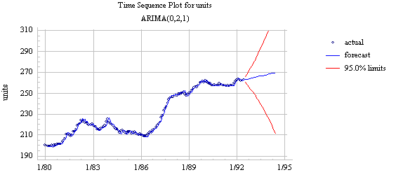
The forecasts have somewhat less of an upward trend than those of the earlier model--because the local trend near the end of the series is slightly less than the average trend over the whole series--but the confidence intervals widen much more rapidly. The model with two orders of differencing assumes that the trend in the series is time-varying, hence it considers the distant future to be much more uncertain than does the model with only one order of differencing.
Which model should we choose? That depends on the assumptions we are comfortable making with respect to the constancy of the trend in the data. The model with only one order of differencing assumes a constant average trend--it is essentially a fine-tuned random walk model with growth--and it therefore makes relatively conservative trend projections. It is also fairly optimistic about the accuracy with which it can forecast more than one period ahead. The model with two orders of differencing assumes a time-varying local trend--it is essentially a linear exponential smoothing model--and its trend projections are somewhat more more fickle. As a general rule in this kind of situation, I would recommend choosing the model with the lower order of differencing, other things being roughly equal. In practice, random-walk or simple-exponential-smoothing models often seem to work better than linear exponential smoothing models.
Mixed models: In most cases, the best model turns out a model that uses either only AR terms or only MA terms, although in some cases a "mixed" model with both AR and MA terms may provide the best fit to the data. However, care must be exercised when fitting mixed models. It is possible for an AR term and an MA term to cancel each other's effects, even though both may appear significant in the model (as judged by the t-statistics of their coefficients). Thus, for example, suppose that the "correct" model for a time series is an ARIMA(0,1,1) model, but instead you fit an ARIMA(1,1,2) model--i.e., you include one additional AR term and one additional MA term. Then the additional terms may end up appearing significant in the model, but internally they may be merely working against each other. The resulting parameter estimates may be ambiguous, and the parameter estimation process may take very many (e.g., more than 10) iterations to converge. Hence:
Unit roots: If a series is grossly under- or overdifferenced--i.e., if a whole order of differencing needs to be added or cancelled, this is often signalled by a "unit root" in the estimated AR or MA coefficients of the model. An AR(1) model is said to have a unit root if the estimated AR(1) coefficient is almost exactly equal to 1. (By "exactly equal " I really mean not significantly different from, in terms of the coefficient's own standard error.) When this happens, it means that the AR(1) term is precisely mimicking a first difference, in which case you should remove the AR(1) term and add an order of differencing instead. (This is exactly what would happen if you fitted an AR(1) model to the undifferenced UNITS series, as noted earlier.) In a higher-order AR model, a unit root exists in the AR part of the model if the sum of the AR coefficients is exactly equal to 1. In this case you should reduce the order of the AR term by 1 and add an order of differencing. A time series with a unit root in the AR coefficients is nonstationary--i.e., it needs a higher order of differencing.
Another symptom of a unit root is that the forecasts of the model may "blow up" or otherwise behave bizarrely. If the time series plot of the longer-term forecasts of the model looks strange, you should check the estimated coefficients of your model for the presence of a unit root.