
As a first step in improving on "naive" forecasting models, nonseasonal patterns and trends can be extrapolated using a moving-average or smoothing model. The basic assumption behind averaging and smoothing models is that the time series is "locally stationary" with a slowly varying mean. Hence, we take a moving (i.e., local) average to estimate the current value of the mean, and use this as the forecast. This can be considered as a compromise between the mean model and the random walk model. The moving average is often called a "smoothed" version of the original series, since short-term averaging has the effect of smoothing out the bumps in the original series. By adjusting the degree of smoothing (i.e., the "width" of the moving average), we can hope to strike some kind of optimal balance between the performance of the mean and random walk models. The simplest kind of averaging model is the....
Simple (equally-weighted) Moving Average:
Ý(t) = (Y(t-1) + Y(t-2) + . . . + Y(t-k))/k
Here, the one-period-ahead forecast Ý(t), made at time t-1, equals the simple average of the last k observations. This average is "centered" at period t-(k+1)/2, which implies that the estimate of the local mean will tend to lag behind the true value of the local mean by about (k+1)/2 periods. Thus, we say the average age of the data in the simple moving average is (k+1)/2 relative to the period for which the forecast is computed: this is the amount of time by which forecasts will tend to lag behind turning points in the data. For example, if you are averaging the last 5 values, the forecasts will be about 3 periods late in responding to turning points. Note that if k=1, the simple moving average (SMA) model is equivalent to the random walk model (without growth). If k is very large (comparable to the length of the estimation period), the SMA model is equivalent to the mean model. As with any parameter of a forecasting model, it is customary to adjust the value of k in order to obtain the best "fit" to the data, i.e., the smallest forecast errors on average.

The random walk model responds very quickly to changes in the series, but in so doing it picks much of the "noise" in the data (the random fluctuations) as well as the "signal" (the local mean). If we instead try a simple moving average of 5 terms, we get a smoother-looking set of forecasts:
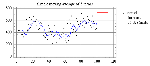
The 5-term simple moving average yields significantly smaller errors than the random walk model in this case. The average age of the data in this forecast is 3 (=(5+1)/2), so that it tends to lag behind turning points by about three periods. (For example, a downturn seems to have occurred at period 21, but the forecasts do not turn around until several periods later.)
Interestingly, the confidence limits computed by Statgraphics for the long-term forecasts of the simple moving average do not get wider as the forecasting horizon increases. This is obviously not correct! Unfortunately, there is no underlying statistical theory that tells us how the confidence intervals ought to widen for this model. If you were going to use this model in practice, you would be well advised to use an empirical estimate of the confidence limits for the longer-horizon forecasts. For example, you could set up a spreadsheet in which the SMA model would be used to forecast 2 steps ahead, 3 steps ahead, etc., within the historical data sample. You could then compute the sample standard deviations of the errors at each forecast horizon, and then construct confidence intervals for longer-term forecasts by adding and subtracting multiples of the appropriate standard deviation.
If we try a 9-term simple moving average, we get even smoother forecasts and more of a lagging effect:

The average age is now 5 periods (=(9+1)/2). If we take a 19-term moving average, the average age increases to 10:

Notice that, indeed, the forecasts are now lagging behind turning points by about 10 periods.
Brown's Simple Exponential Smoothing (exponentially weighted moving average)
The simple moving average model
described above has the undesirable
property that it treats the last k observations equally and completely
ignores all preceding observations. Intuitively, past data should be
discounted
in a more gradual fashion--for example, the most recent observation
should
get a little more weight than 2nd most recent, and the 2nd most recent
should get a little more weight than the 3rd most recent, and so on.
The
simple exponential smoothing (SES) model accomplishes this. Let ![]() denote
a "smoothing constant" (a number between 0 and 1) and let S(t)
denote the value of the smoothed series at period t. The following
formula
is used recursively to update the smoothed series as new observations
are
recorded:
denote
a "smoothing constant" (a number between 0 and 1) and let S(t)
denote the value of the smoothed series at period t. The following
formula
is used recursively to update the smoothed series as new observations
are
recorded:
S(t) = ![]() Y(t) + (1-
Y(t) + (1-![]() )
S(t-1)
)
S(t-1)
Thus, the current smoothed
value is an interpolation between the previous
smoothed value and the current observation, where ![]() controls the
closeness of the interpolated value to the most recent observation. The
forecast for the next period is simply the current
smoothed
value:
controls the
closeness of the interpolated value to the most recent observation. The
forecast for the next period is simply the current
smoothed
value:
Ý(t+1) = S(t)
(Note: we will henceforth use the symbol Ý to stand for a forecast of the time series Y, because Ý is the nearest thing to a "y-hat" that can be displayed on a web page.) Equivalently, we can express the next forecast directly in terms of previous forecasts and previous observations, in any of the following ways:
Ý(t+1) = ![]() Y(t) + (1-
Y(t) + (1-![]() )Ý(t)
...forecast=interpolation between previous forecast and
previous
observation
)Ý(t)
...forecast=interpolation between previous forecast and
previous
observation
Ý(t+1) = Ý(t)
+ ![]() e(t)
...forecast=previous forecast plus fraction
e(t)
...forecast=previous forecast plus fraction ![]() of
previous error, where e(t) = Y(t) - Y(t)
of
previous error, where e(t) = Y(t) - Y(t)
Ý(t+1) = Y(t) - (1- )e(t)
...forecast=previous observation minus fraction 1-
)e(t)
...forecast=previous observation minus fraction 1-![]() of previous error
of previous error
Ý(t+1) = [Y(t) + (1-)Y(t-1)
+ ((1-)^2)Y(t-2) + ((1-)^3)Y(t-3)
+ . . . ] ...forecast=exponentially weighted (i.e. discounted)
moving
average with discount factor 1-![]()
The preceding four equations are all mathematically equivalent--any one of them can be obtained by rearrangement of any of the others. The first equation above is probably the easiest to use if you are implementing the model on a spreadsheet: the forecasting formula fits in a single cell and contains cell references pointing to the previous forecast, the previous observation, and the cell where the value of is stored.
Note that if ![]() =1, the SES
model
is equivalent to a random walk model (without growth). If
=1, the SES
model
is equivalent to a random walk model (without growth). If ![]() =0,
the SES model is equivalent to the mean model, assuming that the first
smoothed value is set equal to the mean.
=0,
the SES model is equivalent to the mean model, assuming that the first
smoothed value is set equal to the mean.
The average age of the data
in the simple-exponential-smoothing forecast
is 1/ relative to the period
for which the forecast is computed. (This is not supposed to be
obvious,
but it can easily be shown by evaluating an infinite series.) Hence,
the
simple moving average forecast tends to lag behind turning points by
about
1/![]() periods. For example, when
periods. For example, when ![]() =
0.5 the lag is 2 periods; when
=
0.5 the lag is 2 periods; when ![]() = 0.2
the lag is 5 periods; when
= 0.2
the lag is 5 periods; when ![]() = 0.1 the
lag is 10 periods, and so on.
= 0.1 the
lag is 10 periods, and so on.
For a given average age (i.e., amount of lag), the simple exponential smoothing (SES) forecast is somewhat superior to the simple moving average (SMA) forecast because it places relatively more weight on the most recent observation--i.e., it is slightly more "responsive" to changes occuring in the recent past.
Another important advantage of
the SES model over the SMA model is that
the SES model uses a smoothing parameter which is continuously
variable,
so it can easily optimized by using a "solver" algorithm to minimize
the mean squared error. The optimal value of ![]() in the SES model for this series turns out to be 0.2961, as shown here:
in the SES model for this series turns out to be 0.2961, as shown here:

The average age of the data in this forecast is 1/0.2961 = 3.4 periods, which is similar to that of a 6-term simple moving average.
The long-term forecasts from the SES model are a horizontal straight line, as in the SMA model and the random walk model without growth. However, note that the confidence intervals computed by Statgraphics now diverge in a reasonable-looking fashion, and that they are substantially narrower than the confidence intervals for the random walk model. The SES model assumes that the series is somewhat "more predictable" than does the random walk model.
An SES model is actually a special case of an ARIMA
model, so the statistical theory of ARIMA models provides a sound basis
for calculating confidence intervals for the SES model. In particular, an
SES model is an ARIMA model with one nonseasonal difference,
an MA(1) term, and no constant term, otherwise known as an
"ARIMA(0,1,1) model without constant". The MA(1) coefficient in the
ARIMA model corresponds to the quantity 1-![]() in the SES model. For example,
if you fit an ARIMA(0,1,1) model without constant to the series
analyzed here, the estimated MA(1) coefficient turns out to be 0.7029,
which is almost exactly one minus 0.2961.
in the SES model. For example,
if you fit an ARIMA(0,1,1) model without constant to the series
analyzed here, the estimated MA(1) coefficient turns out to be 0.7029,
which is almost exactly one minus 0.2961.
It is possible to add the
assumption of a non-zero constant linear trend
to an SES model. To do this in Statgraphics, just specify an ARIMA
model
with one nonseasonal difference and an MA(1) term with a
constant, i.e., an ARIMA(0,1,1) model with
constant.
The long-term forecasts will then have a trend which is equal to the
average
trend observed over the entire estimation period. You cannot do
this in conjunction with seasonal adjustment, because the seasonal
adjustment
options are disabled when the model type is set to ARIMA.
However, you can add a constant
long-term exponential trend to a simple
exponential smoothing model (with or without seasonal adjustment) by
using the inflation adjustment
option in the Forecasting
procedure. The appropriate "inflation" (percentage growth) rate
per period
can be estimated as the slope coefficient in a linear trend model
fitted to the data in conjunction with a natural logarithm
transformation, or it can be based on other, independent information
concerning long-term growth prospects.
Brown's Linear (i.e., double) Exponential Smoothing
If the trend as well as the mean is varying slowly over time, a higher-order smoothing model is needed totrack the varying trend. The simplest time-varying trend model is Brown's linear exponential smoothing (LES) model, which uses two different smoothed series that are centered at different points in time. The forecasting formula is based on an extrapolation of a line through the two centers. (Alternatively, a double application of the simple moving average method can be used to track time-varying trends--see pages 154-158 in your textbook.)
The algebraic form of the linear exponential smoothing model, like that of the simple exponential smoothing model, can be expressed in a number of different but equivalent forms. The "standard" form of this model is usually expressed as follows: Let S' denote the singly-smoothed series obtained by applying simple exponential smoothing to series Y. That is, the value of S' at period t is given by:
S'(t) = Y(t)
+ (1-)S'(t-1)
(Recall that, under simple
exponential smoothing, we would just let
Ý(t+1) = S'(t) at this point.) Then let S" denote the doubly-smoothed
series obtained by applying simple exponential smoothing (using the
same ![]() )
to series S':
)
to series S':
S''(t) = S'(t)
+ (1-)S''(t-1)
Finally, the forecast Ý(t+1) is given by:
Ý(t+1) = a(t) + b(t)
where:
a(t) = 2S'(t) - S''(t) ...the estimated level at period t
b(t) = (/(1-))(S'(t)
- S''(t)) ...the estimated trend at period t.
Forecasts with longer lead times made at period t are obtained by adding multiples of the trend term. For example, the k-period-ahead forecast (i.e., the forecast for Y(t+k) made at period t) would be equal to a(t)+kb(t). For purposes of model-fitting (i.e., calculating forecasts, residuals, and residual statistics over the estimation period), the model can be started up by setting S'(1)=S''(1)=Y(1), i.e., set both smoothed series equal to the observed value at t=1.
A mathematically equivalent form of Brown's linear exponential smoothing model, which emphasizes its non-stationary character and is easier to implement on a spreadsheet, is the following:
Ý(t) = 2Y(t-1) -
Y(t-2) - 2(1-)e(t-1)
+ ((1-)^2)e(t-2)
or equivalently:
Ý(t) - Y(t-1) =
Y(t-1) - Y(t-2) - 2(1-)e(t-1)
+ ((1-)^2)e(t-2)
In other words, the predicted difference at period t (namely Ý(t) - Y(t-1)) is equal to the previous observed difference (namely Y(t-1) - Y(t-2)) minus a weighted difference of the two previous forecast errors.
Caution: this form of the model is rather tricky to start up at the beginning of the estimation period. The following convention is recommended: first set Ý(1) = Y(1), which yields e(1) = 0 (i.e., cheat a bit, and let the first forecast equal the actual first observation), then also set Ý(2) = Y(1), which yields e(2) = Y(2) - Y(1), then continue from this point using the equation above. This would yield the same fitted values as the formula based on S' and S'' if the latter were started up using S'(1) = S''(1) = Y(1).
Once again, you can use your
spreadsheet the "solver" or any
nonlinear least squares algorithm to optimize the value of ![]() .
The optimal value of
.
The optimal value of ![]() in the LES model
fitted to this series by Statgraphics is 0.1607. Note that the
long-term
forecasts of the LES model for this time series appear to track the
local
trend observed in the last 10 periods. Also, the confidence intervals
for
the LES model widen faster than those of the SES model.
in the LES model
fitted to this series by Statgraphics is 0.1607. Note that the
long-term
forecasts of the LES model for this time series appear to track the
local
trend observed in the last 10 periods. Also, the confidence intervals
for
the LES model widen faster than those of the SES model.
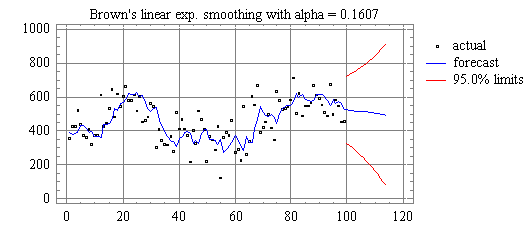
What's best for this particular time series? Here is a model comparison report for the models described above. It appears that the SES model performs better than the SMA models, and LES model is close behind. Whether you choose SES or LES in this case would depend on whether you really believe that the series has a local trend.
Models
------
(A) Random walk
(B) Simple moving average of 5 terms
(C) Simple moving average of 9 terms
(D) Simple exponential smoothing with alpha = 0.2961
(E) Brown's linear exp. smoothing with alpha = 0.1607

Estimation Period
Model  MSE          MAE          MAPE         ME           MPE
------------------------------------------------------------------------
(A)    14825.3      93.2708      23.6152      1.04531      -5.21856
(B)    10329.9      80.6686      20.2747      1.35328      -5.32013
(C)    10826.1      80.2773      20.1534      6.89349      -4.66414
(D)     9776.75     75.0504      18.987       3.27046      -4.84999
(E)    10320.8      77.5989      19.3382      0.553851     -4.67831
Brown's quadratic (i.e., triple) smoothing model ...uses three smoothed series centered at different points in time and extrapolates a parabola through the three centers. This is rarely used in practice, though, since true quadratic trends are rare and the model is highly unstable.
Which type of trend-extrapolation is best: horizontal, linear, or quadratic? Empirical evidence suggests that, if the data have already been adjusted (if necessary) for inflation, then it may be imprudent to extrapolate short-term linear (or worse, quadratic) trends very far into the future. Trends evident today may slacken in the future due to varied causes such as product obsolescence, increased competition, and cyclical downturns or upturns in an industry. For this reason, simple exponential smoothing often performs better out-of-sample than might otherwise be expected, despite its "naive" horizontal trend extrapolation. Damped trend modifications of the linear exponential smoothing model are often used in practice to introduce a note of conservatism into its trend projections--alas, these are not available in Statgraphics.
In principle, it is possible to
calculate confidence intervals around
long-term forecasts produced by exponential smoothing models, by
considering
them as special cases of ARIMA models. (Beware: not all software does
this
correctly. In particular, a number of popular automatic forecasting
programs
use highly suspect methods for calculating confidence intervals for
exponential
smoothing forecasts.) The width of the confidence intervals depends on
(i) the RMS error of the model, (ii) the value of ![]() ,
(iii) the level of smoothing (single, double, or triple); and (iv) the
number of periods ahead you are forecasting. In general, the intervals
spread out faster as
,
(iii) the level of smoothing (single, double, or triple); and (iv) the
number of periods ahead you are forecasting. In general, the intervals
spread out faster as ![]() gets larger and/or
or as the order of smoothing increases from single to double to triple.
We will revisit this subject when we discuss ARIMA models later in the
course.
gets larger and/or
or as the order of smoothing increases from single to double to triple.
We will revisit this subject when we discuss ARIMA models later in the
course.