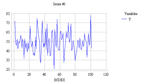


The values of this time series appear to have been independently drawn from a common probability distribution, suggesting that future observations will be drawn from the same distribution. The natural forecast to use for all future values is therefore the sample mean of the past data. The forecasting equation for the mean model is thus:

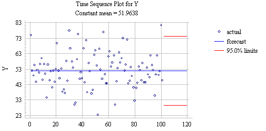
where the estimated constant (alpha) is the sample mean of Y. The estimated standard deviation of the forecast errors, i.e., the forecast standard error, which determines the width of the confidence limits around the forecasts, is approximately equal to (but slightly larger than) the sample standard deviation of Y. (More precisely, the forecast standard error for the mean model is the sample standard deviation multiplied by the square root of 1+1/n, where n is the sample size.) By the usual rule of thumb, an approximate 95% confidence interval for all future forecasts would be the mean plus or minus two standard errors. Here's a plot of the forecasts and confidence intervals, including long-term forecasts for the next 20 values, obtained by selecting the "Mean" forecasting model in SGWIN:

This model may seem too simple and obvious to be of much importance, but it is actually the building block for a number of more sophisticated models, including random walk and ARIMA models. If we can find some mathematical transformation (e.g., differencing, logging, deflating, etc.) that converts the original time series into a stationary white noise series, we can use the mean model to obtain forecasts and confidence limits for the transformed series, and then reverse the transformation to obtain corresponding forecasts and confidence limits for the original series. (Return to top of page.)