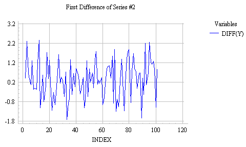

When faced with a time series that shows irregular growth, such as Series #2 analyzed earlier, the best strategy may not be to try to directly predict the level of the series at each period (i.e., the quantity Y(t)). Instead, it may be better to try to predict the change that occurs from one period to the next (i.e., the quantity Y(t)-Y(t-1)). In other words, it may be helpful to look at the first difference of the series, to see if a predictable pattern can be discerned there. For practical purposes, it is just as good to predict the next change as to predict the next level of the series, since the predicted change can always be added to the current level to yield a predicted level. Here's a plot of the first difference of the irregular growth series analyzed above:

Notice that this looks stationary and quite random: a pattern that we previously fitted with the mean model. Hence, the forecasting model suggested by this plot is

...where alpha is the mean of the first difference , i.e., the average change one period to the next. If we rearrange this equation to put Y(t) by itself on the left, we get:

In other words, we predict that this period's value will equal last period's value plus a constant representing the average change between periods. This is the so-called "random walk" model: it assumes that, from one period to the next, the original time series merely takes a random "step" away from its last recorded position. (Think of an inebriated person who steps randomly to the left or right at the same time as he steps forward: the path he traces will be a random walk.)
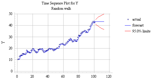
If the constant term (alpha) in the random walk model is zero, it is a random walk without drift. This is the model that SGWIN fits when you specify a "Random walk" on the Model Specification panel in the forecasting procedure. Here is a plot of the Series #2 and the forecast produced by the random-walk model:

Notice that (a) the one-step forecasts within the sample merely "shadow" the observed data, lagging exactly one period behind, and (b) the long-term forecasts outside the sample follow a horizontal straight line anchored on the last observed value. The error measures and residual randomness tests for this model are very much superior to those of the linear trend model, as will be seen below. However, the horizontal appearance of the long-term forecasts is rather unsatisfactory if we believe that the upward trend observed in the past is genuine. (Return to top of page.)
Random walk with drift: If the series being fitted by a random walk model has an average upward (or downward) trend that is expected to continue in the future, you should include a non-zero constant term in the model--i.e., assume that the random walk undergoes "drift." To add a non-zero constant drift term to the random walk model in SGWIN, you can just check the "constant" box on the Model Options panel after specifying a random walk model. This works fine if you are not holding out any data for validation, but unfortunately there is a bug in this feature that surfaces when you are holding out data: the drift term is still estimated from the entire sample. (You'll notice that the forecasts do not change at all when more or fewer data points are held out.) To fit a random-walk-with-drift model with data held out for validation, you must specify it as a special case of an ARIMA model. ARIMA models are a very general class of forecasting models that includes random walk models and more elaborate models whose forecasting equations may include lags of the differenced time series (so-called auto-regressive or "AR" terms) and/or lags of the forecast errors (so-called moving-average or "MA" terms).
To specify the random walk model with non-zero constant drift, (i) select "ARIMA" as the model type, (ii) set the order of non-seasonal differencing to 1, (iii) set all the AR, MA, SAR, and SMA terms to zero (the default setting is AR=1: change this to zero), and (iv) leave the "constant" box checked (i.e., do estimate a constant). By choosing these settings, you are simply applying the constant (mean) forecasting model to the first difference of the series, although SGWIN will "undifference" the forecasts for you in the plots and output reports. In ARIMA terminology, this is a "(0,1,0) model with constant," where the numbers in parentheses refer to the number of AR terms, the number of nonseasonal differences, the number of MA terms, respectively. Here's the result of specifying this model for Series #2:

This picture looks much the same as the previous one, except that the long-term forecasts now trend upward. The slope of the forecasts is merely the average monthly difference that was calculated inside the sample, which is 0.259231. (This is the "alpha" term in the forecasting equation, and it shows up as the estimated constant in the Analysis Summary report for the model.) This value is very close--but not quite identical--to the slope of the forecasts in the linear trend model, which was 0.258761. However, the intercept of the out-of-sample forecasts of the random walk model is always reanchored so that that the forecasts extend from the last observed data point, rather some point fixed in the past.
If we look at the Model Comparison report for the three models (linear trend, random walk, and random walk with constant), we see that the last model is indeed the best, both in-sample and out-of-sample.
An advantage to using the ARIMA model option to fit a random walk model is that it easily allows you to add terms to correct the model for autocorrelation in the residuals, if this should be necessary. In particular, if the random walk model has significant positive autocorrelation in the residuals at lag 1, you should try setting AR=1, which yields a so-called ARIMA(1,1,0) model. On the other hand, if the random walk model has significant negative autocorrelation in the residuals at lag 1, you should try setting MA=1, which yields a so-called ARIMA(0,1,1) model, which is essentially the same as a simple exponential smoothing model. We will discuss these model types and autocorrelation-correction strategies in more depth later in the course.