 Averaging and
smoothing models
Averaging and
smoothing models
Notes
on forecasting with moving averages (pdf)
Moving average and
exponential smoothing models
Slides
on inflation and seasonal adjustment and Winters seasonal exponential smoothing
Spreadsheet implementation of seasonal adjustment and
exponential smoothing
Equations
for the smoothing models (SAS web site)
Moving average and
exponential smoothing models
Simple moving average
model
Brown’s simple exponential smoothing model
Brown’s linear exponential smoothing model
Holt’s linear exponential smoothing model
As a first
step in moving beyond mean models, random walk models, and linear trend models,
nonseasonal patterns and trends can be extrapolated using a moving-average
or smoothing model. The basic assumption behind averaging and smoothing
models is that the time series is locally stationary with a slowly varying
mean. Hence, we take a moving (local) average to estimate the current
value of the mean and then use that as the forecast for the near future. This
can be considered as a compromise between the mean model and the
random-walk-without-drift-model. The same strategy can be used to estimate and
extrapolate a local trend. A moving
average is often called a "smoothed" version of the original series
because short-term averaging has the effect of smoothing out the bumps in the
original series. By adjusting the degree of smoothing (the width of the moving
average), we can hope to strike some kind of optimal balance between the
performance of the mean and random walk models. The simplest kind of averaging
model is the....
Simple
(equally-weighted) Moving Average:
The forecast
for the value of Y at time t+1 that is made at time t equals the simple average
of the most recent m observations:
![]()
(Here and elsewhere I will use the symbol
“Y-hat” to stand for a forecast of the time series Y made at the
earliest possible prior date by a given model.) This average is centered at period t-(m+1)/2, which
implies that the estimate of the local mean will tend to lag behind the true
value of the local mean by about (m+1)/2 periods. Thus, we say the average age of the data in the simple
moving average is (m+1)/2 relative to the period for which the forecast is
computed: this is the amount of time by which forecasts will tend to lag
behind turning points in the data. For example, if you are averaging the
last 5 values, the forecasts will be about 3 periods late in responding to
turning points. Note that if m=1, the simple moving average (SMA) model is
equivalent to the random walk model (without growth). If m is very large
(comparable to the length of the estimation period), the SMA model is
equivalent to the mean model. As with any parameter of a forecasting model, it
is customary to adjust the value of k in order to obtain the best "fit"
to the data, i.e., the smallest forecast errors on average.
Here is an example of a series which
appears to exhibit random fluctuations around a slowly-varying mean. First,
let's try to fit it with a random walk model, which is equivalent to a simple
moving average of 1 term:
The random
walk model responds very quickly to changes in the series, but in so doing it
picks much of the "noise" in the data (the random fluctuations) as
well as the "signal" (the local mean). If we instead try a simple
moving average of 5 terms, we get a smoother-looking set of forecasts:
The 5-term
simple moving average yields significantly smaller errors than the random walk
model in this case. The average age of the data in this forecast is 3
(=(5+1)/2), so that it tends to lag behind turning points by about three
periods. (For example, a downturn seems to have occurred at period 21, but the
forecasts do not turn around until several periods later.)
Notice that the long-term forecasts
from the SMA model are a horizontal straight line, just as in the
random walk model. Thus, the SMA model assumes that there is no trend in
the data. However, whereas the forecasts from the random walk model are simply
equal to the last observed value, the forecasts from the SMA model are equal to
a weighted average of recent values.
The confidence
limits computed by Statgraphics for the long-term forecasts of the simple
moving average do not get wider as the forecasting horizon increases.
This is obviously not correct! Unfortunately, there is no underlying
statistical theory that tells us how the confidence intervals ought to widen
for this model. However, it is not
too hard to calculate empirical
estimates of the confidence limits for the longer-horizon forecasts. For
example, you could set up a spreadsheet in which the SMA model would be used to
forecast 2 steps ahead, 3 steps ahead, etc., within the historical data sample.
You could then compute the sample standard deviations of the errors at each
forecast horizon, and then construct confidence intervals for longer-term
forecasts by adding and subtracting multiples of the appropriate standard
deviation.
If we try
a 9-term simple moving average, we get even smoother forecasts and more of a
lagging effect:
The
average age is now 5 periods (=(9+1)/2). If we take a 19-term moving average,
the average age increases to 10:

Notice
that, indeed, the forecasts are now lagging behind turning points by about 10
periods.
Which
amount of smoothing is best for this series? Here is a table that compares their
error statistics, also including a 3-term average:

Model C,
the 5-term moving average, yields the lowest value of RMSE by a small margin
over the 3-term and 9-term averages, and their other stats are nearly
identical. So, among models with
very similar error statistics, we can choose whether we would prefer a little
more responsiveness or a little more smoothness in the forecasts. (Return to top of page.)
Brown's
Simple Exponential Smoothing (exponentially weighted moving average)
The simple
moving average model described above has the undesirable property that it
treats the last k observations equally and completely ignores all preceding
observations. Intuitively, past data should be discounted in a more gradual
fashion--for example, the most recent observation should get a little more
weight than 2nd most recent, and the 2nd most recent should get a little more
weight than the 3rd most recent, and so on. The simple exponential smoothing
(SES) model accomplishes this.
Let α denote a "smoothing
constant" (a number between 0 and 1).
One way to write the model is to define a series L that represents the
current level (i.e., local mean value) of the series as estimated from data up
to the present. The value of
L at time t is computed recursively from its own previous value like this:
Lt
= αYt +
(1-α) Lt-1
Thus, the current smoothed value is an
interpolation between the previous smoothed value and the current observation,
where α controls the
closeness of the interpolated value to the most recent observation. The forecast
for the next period is simply the current smoothed value:
![]()
Equivalently, we can express the next
forecast directly in terms of previous forecasts and previous observations, in
any of the following equivalent versions.
In the first version, the forecast is an interpolation between previous forecast
and previous observation:
![]()
In the second version, the next forecast is
obtained by adjusting the previous forecast in the direction of the
previous error by a fractional amount
α:
![]()
where
![]()
is the error made at time t. In the third version, the forecast is an exponentially
weighted (i.e. discounted) moving average with discount factor 1-α:
![]()
The interpolation version of the
forecasting formula is the simplest to use if you are implementing the model on
a spreadsheet: it fits in a single cell and contains cell references pointing
to the previous forecast, the previous observation, and the cell where the
value of α is stored.
Note that
if α=1, the SES model
is equivalent to a random walk model (without growth). If α=0, the SES model is equivalent to the mean
model, assuming that the first smoothed value is set equal to the mean. (Return to top of page.)
The
average age of the data in the simple-exponential-smoothing forecast is 1/α relative to the
period for which the forecast is computed. (This is not supposed to be obvious,
but it can easily be shown by evaluating an infinite series.) Hence, the simple
moving average forecast tends to lag behind turning points by about 1/α periods. For example, when α=0.5 the lag is 2 periods; when α=0.2 the lag is 5 periods; when α=0.1 the lag is 10 periods, and so on.
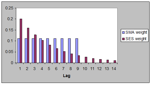
For a
given average age (i.e., amount of lag), the simple exponential smoothing (SES)
forecast is somewhat superior to the simple moving average (SMA) forecast
because it places relatively more weight on the most recent observation--i.e.,
it is slightly more "responsive" to changes occuring in the recent
past. For example, an SMA model with 9 terms and an SES model
with α=0.2 both have an
average age of 5 for the data in their forecasts, but the SES model
puts more weight on the last 3 values than does the SMA model and at the same
time it doesn’t entirely “forget” about values more than 9
periods old, as shown in this chart:
![]()
Another
important advantage of the SES model over the SMA model is that the SES model
uses a smoothing parameter which is continuously variable, so it can easily
optimized by using a "solver" algorithm to minimize the mean squared
error. The optimal value of α in the SES model for this series turns out
to be 0.2961, as shown here:
The
average age of the data in this forecast is 1/0.2961 = 3.4 periods, which is
similar to that of a 6-term simple moving average.
The
long-term forecasts from the SES model are a horizontal straight line,
as in the SMA model and the random walk model without growth. However, note
that the confidence intervals computed by Statgraphics now diverge in a
reasonable-looking fashion, and that they are substantially narrower than the
confidence intervals for the random walk model. The SES model assumes that the
series is somewhat "more predictable" than does the random walk
model.
An SES
model is actually a special case of an ARIMA model, so the statistical
theory of ARIMA models provides a sound basis for calculating confidence
intervals for the SES model. In particular, an SES model is an ARIMA model
with one nonseasonal difference, an MA(1) term, and no constant term,
otherwise known as an "ARIMA(0,1,1) model without constant". The
MA(1) coefficient in the ARIMA model corresponds to the quantity 1-α in the SES model. For example, if you fit
an ARIMA(0,1,1) model without constant to the series analyzed here, the
estimated MA(1) coefficient turns out to be 0.7029, which is almost exactly one
minus 0.2961.
It is
possible to add the assumption of a non-zero constant linear trend to an
SES model. To do this, just specify an ARIMA model with one nonseasonal
difference and an MA(1) term with a constant, i.e., an ARIMA(0,1,1)
model with constant. The long-term forecasts will then have a trend
which is equal to the average trend observed over the entire estimation period.
You cannot do this in conjunction with seasonal adjustment, because the
seasonal adjustment options are disabled when the model type is set to
ARIMA. However, you can add a constant long-term exponential trend
to a simple exponential smoothing model (with or without seasonal adjustment)
by using the inflation adjustment option in the Forecasting
procedure. The appropriate "inflation" (percentage growth) rate
per period can be estimated as the slope coefficient in a linear trend model
fitted to the data in conjunction with a natural logarithm transformation, or
it can be based on other, independent information concerning long-term growth
prospects. (Return
to top of page.)
Brown's Linear (i.e., double)
Exponential Smoothing
The SMA models and SES models assume that there is no trend of any kind in the
data (which is usually OK or at least not-too-bad for 1-step-ahead forecasts when
the data is relatively noisy), and they can be modified to incorporate a
constant linear trend as shown above.
What about short-term trends?
If a series displays a varying rate of growth or a cyclical pattern that
stands out clearly against the noise, and if there is a need to forecast more
than 1 period ahead, then estimation of a local trend might also be an
issue. The simple exponential
smoothing model can be generalized to obtain a linear exponential smoothing (LES) model that computes local estimates of both level and
trend.
The simplest time-varying trend model is Brown's linear exponential
smoothing model, which uses two different smoothed series
that are centered at different points in time. The forecasting formula is based on an
extrapolation of a line through the two centers. (A more sophisticated version of
this model, Holt’s, is discussed below.)
The algebraic form of Brown’s linear exponential
smoothing model, like that of the simple exponential smoothing model, can be
expressed in a number of different but equivalent forms. The
"standard" form of this model is usually expressed as follows: Let S'
denote the singly-smoothed series obtained by applying simple
exponential smoothing to series Y. That is, the value of S' at period t is
given by:
![]()
(Recall that, under simple
exponential smoothing, this would be the forecast for Y at period t+1.) Then
let S" denote the doubly-smoothed series obtained by applying
simple exponential smoothing (using the same α) to series S':
![]()
Finally, the forecast for Yt+k, for any k>1, is given by:
![]()
where:
![]()
...is the estimated level at
period t, and
![]()
...is the
estimated trend at period t.
For purposes of model-fitting (i.e., calculating forecasts,
residuals, and residual statistics over the estimation period), the model can
be started up by setting S'1 =
S''1 = Y1, i.e., set both smoothed
series equal to the observed value at t=1.
(Return to top of page.)
A mathematically equivalent form of Brown's linear
exponential smoothing model, which emphasizes its non-stationary character and
is easier to implement on a spreadsheet, is the following:
![]()
or equivalently:
![]()
In other words, the predicted
difference at period t is equal to the previous observed difference minus
a weighted difference of the two previous forecast errors.
Caution: this form of the model is rather
tricky to start up at the beginning of the estimation period. The following
convention is recommended:
![]()
This yields e1 = 0 (i.e., cheat a bit, and let
the first forecast equal the actual first observation), and e2 =
Y2 – Y1, after which forecasts are generated
using the equation above. This yields the same fitted values as the formula
based on S' and S'' if the latter were started up using S'1 = S''1 =
Y1. This
version of the model is used on the next page that illustrates a combination of exponential
smoothing with seasonal adjustment.
Holt’s
Linear Exponential Smoothing
Brown’s LES model computes local
estimates of level and trend by smoothing the recent data, but the fact that it
does so with a single smoothing parameter places a constraint on the data
patterns that it is able to fit:
the level and trend are not allowed to vary at independent rates. Holt’s LES model addresses this
issue by including two smoothing
constants, one for the level and one for the trend. At any time t, as in Brown’s
model, the there is an estimate Lt of the local level and an
estimate Tt of the local trend.
Here they are computed recursively from the value of Y observed at time
t and the previous estimates of the level and trend by two equations that apply
exponential smoothing to them separately.
If the estimated level and trend at time
t-1 are Lt‑1 and Tt-1, respectively, then the
forecast for Yt that would have been made at time t-1 is equal
to Lt-1+Tt-1.
When the actual value is observed, the updated estimate of the level is
computed recursively by interpolating between Yt and its
forecast, Lt-1+Tt-1, using weights of α and 1-α:
![]()
The change in the estimated level, namely Lt
‑ Lt‑1, can be interpreted as a noisy measurement
of the trend at time t. The updated
estimate of the trend is then computed recursively by interpolating between Lt
‑ Lt‑1 and the previous estimate of the trend, Tt-1,
using weights of β and 1-β:
![]()
Finally, the forecasts for the near future
that are made from time t are obtained by extrapolation of the updated level
and trend:
![]()
The interpretation of the trend-smoothing
constant β is analogous to that of the level-smoothing constant
α. Models with small values of β
assume that the trend changes only very slowly over time, while models with
larger β assume that it is changing more rapidly. A model with a large β believes
that the distant future is very uncertain, because errors in trend-estimation
become quite important when forecasting more than one period ahead. (Return to top of page.)
The smoothing constants α and β can be
estimated in the usual way by minimizing the mean squared error of the
1-step-ahead forecasts. When this
done in Statgraphics, the estimates turn out to be α =0.3048 and β
=0.008. The very small value of
β means that the model assumes very little change in the trend from one
period to the next, so basically this model is trying to estimate a long-term
trend. By analogy with the
notion of the average age of the data that is used in estimating the local
level of the series, the average age of the data that is used in estimating the
local trend is proportional to 1/ β, although not exactly equal to it. In
this case that turns out to be 1/0.006 = 125. This isn’t a very precise number
inasmuch as the accuracy of the estimate of β isn’t really 3 decimal
places, but it is of the same general order of magnitude as the sample size of
100, so this model is averaging over quite a lot of history in estimating the
trend. The forecast plot
below shows that the LES model estimates a slightly larger local trend at the
end of the series than the constant trend estimated in the SES+trend
model. Also, the estimated value of
α
is almost identical to the one obtained by fitting the SES model with or
without trend, so this is almost the same model.


Now, do these look like reasonable
forecasts for a model that is supposed to be estimating a local trend? If you “eyeball” this plot,
it looks as though the local trend has turned downward at the end of the
series! What has happened? The parameters of this model have been estimated
by minimizing the squared error of 1-step-ahead forecasts, not longer-term
forecasts, in which case the trend doesn’t make a lot of difference. If all you are looking at are
1-step-ahead errors, you are not seeing the bigger picture of trends over (say)
10 or 20 periods. In order to get
this model more in tune with our eyeball extrapolation of the data, we can
manually adjust the trend-smoothing constant so that it uses a shorter baseline
for trend estimation. For
example, if we choose to set β =0.1, then the average age of the data used
in estimating the local trend is 10 periods, which means that we are averaging
the trend over that last 20 periods or so.
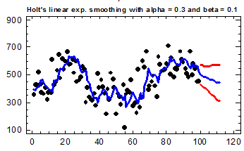
Here’s what the forecast plot looks like if we set β =0.1
while keeping α
=0.3. This looks intuitively
reasonable for this series, although it is probably dangerous to extrapolate this
trend any more than 10 periods in the future.

What about the error stats? Here is a model comparison for the two
models shown above as well as three SES models. The optimal value of α.for the SES model
is approximately 0.3, but similar results (with slightly more or less
responsiveness, respectively) are obtained with 0.5 and 0.2.
Models
(A) Holt's linear exp. smoothing with alpha = 0.3048
and beta = 0.008
(B) Holt's linear exp. smoothing with alpha = 0.3 and
beta = 0.1
(C) Simple exponential smoothing with alpha = 0.5
(D) Simple exponential smoothing with alpha = 0.3
(E) Simple exponential smoothing with alpha = 0.2
Estimation Period
|
Model |
RMSE |
MAE |
MAPE |
ME |
MPE |
|
(A) |
98.9302 |
76.3795 |
16.418 |
-6.58179 |
-7.0742 |
|
(B) |
100.863 |
78.3464 |
16.047 |
-3.78268 |
-5.63482 |
|
(C) |
101.053 |
76.7164 |
14.605 |
1.70418 |
-4.94903 |
|
(D) |
98.3782 |
75.0551 |
18.9899 |
3.21634 |
-4.85287 |
|
(E) |
99.5981 |
76.3239 |
12.528 |
5.20827 |
-4.7815 |
|
Model |
RMSE |
RUNS |
RUNM |
AUTO |
MEAN |
VAR |
|
(A) |
98.9302 |
OK |
OK |
OK |
OK |
OK |
|
(B) |
100.863 |
OK |
OK |
OK |
OK |
OK |
|
(C) |
101.053 |
OK |
OK |
OK |
OK |
OK |
|
(D) |
98.3782 |
OK |
OK |
OK |
OK |
OK |
|
(E) |
99.5981 |
OK |
* |
OK |
OK |
OK |
Their
stats are nearly identical, so we really can’t make the choice on the
basis of 1-step-ahead forecast errors within the data sample. We have to fall back on other
considerations. If we strongly
believe that it makes sense to base the current trend estimate on what has
happened over the last 20 periods or so, we can make a case for the LES model
with α
= 0.3 and β = 0.1. If we want
to be agnostic about whether there is a local trend, then one of the SES models
might be easier to explain and would also give more middle-of-the-road
forecasts for the next 5 or 10 periods.
(Return to top of page.)
Which type of
trend-extrapolation is best: horizontal or linear? Empirical evidence
suggests that, if the data have already been adjusted (if necessary) for
inflation, then it may be imprudent to extrapolate short-term linear trends
very far into the future. Trends evident today may slacken in the future due to
varied causes such as product obsolescence, increased competition, and cyclical
downturns or upturns in an industry. For this reason, simple exponential
smoothing often performs better out-of-sample than might otherwise be expected,
despite its "naive" horizontal trend extrapolation. Damped trend modifications of the
linear exponential smoothing model are also often used in practice to introduce
a note of conservatism into its trend projections. The damped-trend LES model can be
implemented as a special case of an ARIMA model, in particular, an ARIMA(1,1,2) model.
It is possible to
calculate confidence intervals around long-term forecasts produced by
exponential smoothing models, by considering them as special cases of ARIMA models. (Beware: not all software calculates
confidence intervals for these models correctly.) The width of the confidence intervals
depends on (i) the RMS error of the model, (ii) the type of smoothing (simple
or linear); (iii) the value(s) of
the smoothing constant(s); and (iv) the number of periods ahead you are forecasting.
In general, the intervals spread out faster as α gets larger in the
SES model and they spread out much faster when linear rather than simple
smoothing is used. This topic is
discussed further in the ARIMA models section of the notes. (Return to top of page.)
Go on to next topic: spreadsheet implementation of seasonal
adjustment and exponential smoothing