Statistics
review and the simplest forecasting model: the sample mean (pdf)
Notes on the random
walk model (pdf)
Mean (constant) model
Linear trend model
Random walk model
Geometric random walk model
Three types of forecasts: estimation, validation, and the future
Three types of forecasts: estimation,
validation, and the future
A good way
to test the assumptions of a model and to realistically compare its forecasting performance
against other models is to perform out-of-sample validation, which means
to withhold some of the sample data from the model identification and
estimation process, then use the model to make predictions for the hold-out
data in order to see how accurate they are and to determine whether the statistics of their errors are similar to those that the model made within the sample of data that was fitted. In the
Forecasting procedure in Statgraphics, you are given the option to specify a number
of data points to hold out for validation and a number of forecasts
to generate into the future. The data which are not held out are used to
estimate the parameters of the model. The model is then tested on data in the
validation period, and forecasts are generated beyond the end of the
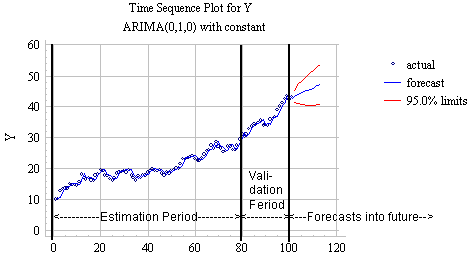
estimation and validation periods. For example, consider a hypothetical time
series Y of which a sample of 100 observations is available, as shown in the
chart below. Suppose that a random-walk-with-drift
model (which is specified as an "ARIMA(0,1,0) with constant" model in
Statgraphics) is fitted to this series.
If the last 20 values are held out for validation and 12 forecasts for
the future are generated, the results look like this:

In
general, the data in the estimation period are used to help select the
model and to estimate its parameters. Forecasts made in this period are
not completely "honest" because data on both sides of each observation
are used to help determine the forecast. The one-step-ahead forecasts made in
this period are usually called fitted values. (They are said to be
"fitted" because our software estimates the parameters of the model
so as to "fit" them as well as possible in a mean-squared-error
sense.) The corresponding forecast errors are called residuals. The
residual statistics (MSE, MAE, MAPE) may understate the magnitudes of the
errors that will be made when the model is used to predict the future, because
it is possible that the data have been overfitted--i.e, by relentlessly
minimizing the mean squared error, the model may have inadvertently fitted some
of the "noise" in the estimation period as well as the
"signal." Overfitting is especially likely to occur when either (a) a
model with a large number of parameters (e.g., a model using seasonal
adjustment) has been fitted to a small sample of data and/or (b) the model has
been selected from a large set of potential models precisely by minimizing the
mean squared error in the estimation period (e.g., when stepwise or all-subsets
regression has been used with a large set of potential regressors).
The data
in the validation period are held out during parameter
estimation, and if you are careful you will also withhold these values during
the exploratory phase of analysis when you select your model. One-step-ahead
forecasts made in this period are often called backtests. Ideally, these
are "honest" forecasts and their error statistics are representative
of errors that will be made in forecasting the future. However, if you test a
great number of models and choose the model whose errors are smallest in the
validation period, you may end up overfitting the data within the validation
period as well as in the estimation period.
In
Statgraphics, the statistics of the forecast errors in the validation period
are reported alongside the statistics of the forecast errors in the estimation
period, so that you can compare them. For example, the Analysis Summary report
for the random walk model with drift looked like this:
Forecast
model selected: ARIMA(0,1,0) with constant
Number of forecasts generated: 12
Number of periods withheld for validation: 20
Estimation Validation
Statistic
Period Period
--------------------------------------------
MSE
0.886679 1.02186
MAE
0.762752 0.835759
MAPE
3.85985 2.263
ME
-0.00515478 0.381454
MPE
-0.0865215 1.00468
If the data have not been badly
overfitted, the error measures in the validation period should be similar to
those in the estimation period, although they are often at least slightly
larger. Here we see that the MSE in the validation period is indeed slightly
larger than in the estimation period: 1.02 versus 0.89.
Holding data out
for validation purposes is probably the single most important diagnostic test
of a model: it
gives the best indication of the accuracy that can be expected when forecasting
the future. If you have the luxury of large quantities of data, I recommend
that you hold out at least 20% of your data for validation purposes. If you really
have a lot of data, you might even try holding out 50%--i.e., select and fit
the model to one-half of the data. then validate it on the other half. In the
case of regression models, you can run this exercise both ways and compare
coefficient estimates as well as error statistics between the first half and
last half. Ideally these should be in general agreement as well. When you're
ready to forecast the future in real time, you should of course use all
the available data for estimation, so that the most recent data is used. Alas,
it is difficult to properly validate a model if data is in short supply. For
example, if you have only 20 data points, then you cannot afford to hold out
very many for validation, and your sample size for the validation period may be
too small to be a reliable indicator of future forecasting performance.
Forecasts into the
future are
"true" forecasts that are made for time periods beyond the end of the
available data. For a model which is purely extrapolative in nature
(i.e., which it forecasts a time series entirely from its own history), it is
possible to extend the forecasts an arbitrary number of periods into the future
by "bootstrapping" the model: first a one-period-ahead forecast is
made, then the one-period-ahead forecast is treated as a data point and the
model is cranked ahead to produce a two-period-ahead forecast, and so on as far
as you wish.
Most forecasting
software is capable of performing this kind of extrapolation automatically and
also calculating confidence intervals for the forecasts. (The 95%
confidence interval is roughly equal to the forecast plus-or-minus two times
the estimated standard deviation of the forecast error at each period.) The
confidence intervals typically widen as the forecast horizon increases,
due to the expected build-up of error in the bootstrapping process. The rate at
which the confidence intervals widen will in general be a function of the type
of forecasting model selected. Models may differ in their assumptions
about the intrinsic variability of the data, and these assumptions are not
necessarily correct. Therefore, the model with the tightest confidence
intervals is not always the best model: a bad model does not always know
it is a bad model! For example, the linear trend model assumes that the
data will vary randomly around a fixed trend line, and its confidence intervals
therefore widen very little as the forecast horizon increases. (They only
reason that they widen at all is because of uncertainty in the slope and
intercept coefficients based on small samples of data.) As we have seen, this
assumption is often inappropriate, and therefore the confidence intervals for
the linear trend model are usually overly optimistic (i.e., too narrow).
The confidence intervals for the random walk model diverge in a pattern that is proportional to the square root of the forecast horizon (a sideways parabola). This "square root of time" rule follows from the fact that the variance of the errors in the random walk model grows linearly: the variance of the two-step-ahead forecast error is exactly twice the variance of the one-step-head forecast error, the variance of the three-step-ahead forecast error is exactly three times the variance of the one-step-ahead forecast error, and so on. After n steps into the future, the variance of the forecast error is n times the one-step-ahead error variance, and since the standard deviation of the forecast errors is the square root of the variance, the standard deviation of the n-step ahead forecast error is proportional to the square root of n for the random walk model.
