 Simple forecasting models
Statistics
review and the simplest forecasting model: the sample mean (pdf)
Notes on the random
walk model (pdf)
Mean (constant) model
Linear trend model
Random walk model
Geometric random walk model
Three types of forecasts: estimation, validation, and the
future
Mean (constant) model
The most elementary case of
statistical forecasting is that of predicting a variable whose values are independently and identically randomly
distributed ("i.i.d").
For example, consider a variable X1 for which a sample of size 30 has been
observed and whose values are plotted below versus the row number in the data
file:
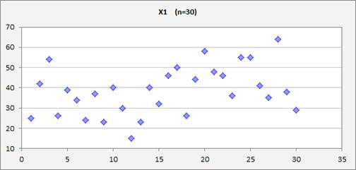
(The file containing this data and the model below can be found here.) Suppose that a 31st
value is going to be observed at some point in the future, and we would like to
make a forecast for it in advance. How should we do it? If the values of X1 are independently
and identically distributed, then the most natural forecast to use is the sample mean of the historical data. Why the sample mean? Because by definition it is an unbiased predictor and also it minimizes the mean squared forecasting
error regardless of the shape of the probability distribution. The sample mean has the property that it
is the value around which the sum of squared deviations of the sample data is
minimized. This is not obvious, but
it is easily proved with a little calculus. This very simple forecasting model will
be called the "mean model"
or "constant model." The sample mean of X1 is 38.5, so according to the mean model,
we should predict that its 31st value (and all future values) will
be 38.5.
Now, how accurate is this estimate of the
mean, based on the limited sample of data?
That is measured by the standard
error of the mean, which is the estimated standard deviation of the error
in the sample mean. The standard error of the mean is equal
to the sample standard deviation divided by the square root of the sample
size. Here the sample standard deviation is
12.0, and the sample size is 30, so the standard error of the mean is 12/SQRT(30) = 2.2. By virtue of the Central Limit Theorem,
we can assume the error in the estimating the mean to be approximately normally
distributed for a sample this large, regardless of the distribution of the
random variable itself, and on this basis we can construct confidence intervals
for the mean. In general, a confidence interval for a parameter
estimate is equal to its point value plus or minus an appropriate number of
standard errors. The
appropriate number is the so-called
critical t-value and it is determined by the desired confidence level and by the number
of degrees of freedom for error (the sample size minus the number of
parameters estimated from it). The T.INV.2T function in Excel can be used
to compute critical t-values for 2-tailed confidence intervals. For a 95% confidence interval for the
mean, the critical t-value is T.INV.2T(0.05,
n-1) where n is the sample size.
Here the sample size is 30, so the critical t-value for a 95% confidence
interval is T.INV.2T(0.05, 29), which is 2.05. A 95% confidence interval for the mean
is therefore 38.5 plus or minus 2.05
times 2.2, which is [34.0, 43.0].
For samples of this size or larger, the
critical t-value for a 95% confidence interval is always very close to 2 (it
approaches 1.96 in the limit as the sample size goes to infinity), so a 95%
confidence interval is roughly "plus or minus 2 standard errors"
under a wide range of conditions. (Return to top of page.)
Next, how
accurate is the estimated mean as a forecast
for the next value of X1 that will be observed? In general, when forecasts are being
made for future values of random variables, there are two sources of error: (i)
intrinsically unexplainable variations ("noise") in the data, and
(ii) errors in the parameter estimates upon which the forecasts are based. For the mean model, the magnitudes
of these two sources of error are measured by the sample standard deviation and
the standard error of the mean respectively, and together they determine the standard error of the forecast, which
is the estimated standard deviation of the error in the forecast. (The error in the forecast is defined as
the observed value minus the forecast.)
Specifically, the standard error of a forecast from the mean model is equal
to the square root of {the square of the sample standard deviation plus the
square of the standard error of the mean}.
Because the standard error of the mean is just the sample standard
deviation divided by the square root of n, it follows that, for the mean model, the standard error of
the forecast is equal to the sample standard deviation multiplied by the square
root of 1+1/n. In the case of X1, the standard error of the forecast
is therefore 12.0 x SQRT(1+1/30) = 12.2,
which is only slightly larger than the sample standard deviation.
The
standard error of the forecast can used to determine confidence intervals for
forecasts in the usual way: a confidence interval for a forecast is the
point forecast plus-or-minus the appropriate critical t-value times the
standard error of the forecast.
The critical t-value is the same as the one used to calculate a
confidence interval for the mean. So, the 95% confidence interval for the
forecast in this model is 38.5
plus-or-minus 2.05 times 12.2, which is [13.5, 63.5] Here we must be a
bit careful, though. The formula for calculating a symmetric
2-tailed confidence interval is
based on an assumption of normally distributed errors. But the error in a forecast based on the
mean model is normally distributed only if
the variable itself is normally distributed. (We cannot automatically appeal to the
Central Limit Theorem here, because what is being predicted is a single
observation, not the mean of many observations.) So, to be careful, we ought to look at
the probability distribution of the
forecast errors, as revealed by charts and statistics that test for
normality of the distribution.
The
accompanying Excel
file in which this analysis was carried out with RegressIt includes the following table and
chart which show the forecasts for X1 produced by the model, together with the
95% confidence interval around the forecast for observation #31. (It also includes various plots and
statistical tests of the errors.)
![]()
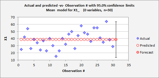
The
forecast and the confidence interval look somewhat reasonable (if a little boring),
although they rest on strong assumptions, namely that the values of X1 are
independently and identically normally distributed. It would be good to look
deeper into these assumptions, and this will be done in the section on the linear trend model.
A few words about confidence levels: It is conventional to use 95% as the
default confidence level when reporting confidence intervals for parameter estimates
or forecasts, although there is no magical signficance attached to this
value. It is merely an arbitrary
standard of "very confident but not certain". The number 0.95 is close to 1 but not so
close as to be visually indistinguishable, and a 1-out-of-20 chance of a
surprise is not too tiny to think carefully about. (Most persons have trouble in
appreciating the relative importance of very
small probabilities, though, such as a 1-out-of-100 or 1-out-of-1000 chance.) Also, 2 is a nice round number for
a critical t-value. But in some
situations it may be helpful to compute and plot confidence intervals for some
other confidence level, say, 90% or 99% or only 50%, particularly when the
setting is one of forecasting rather than inference about parameter
values. The critical t-value for a 50% confidence interval is approximately
2/3, so a 50% confidence interval is one-third the width of a 95% confidence
interval. Here's what the
forecast chart for the mean model for X1 looks like with 50% confidence limits:
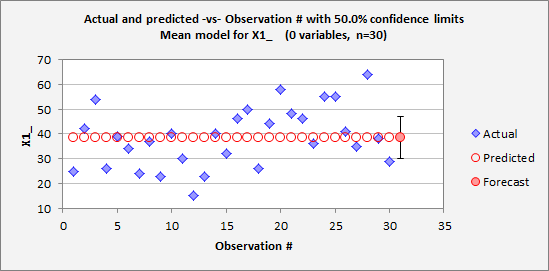
The nice thing about a 50% confidence
interval is that it is a "coin flip" as to whether the true value
will fall inside or outside of it, which is extremely easy to think about. Also, confidence intervals for forecasts
at high levels of confidence tend to be so wide as to not be very informative
on a plot, particularly when sample sizes are small. The 95%
confidence interval for a forecast from the mean model is often approximately the range of the sample data, as
in the first chart above. 50%
intervals are often more helpful as visual reference points, particularly when
comparing the degree of overlap between forecasts produced by different
models. In general, the
consequences of error in the decision problem at hand, as well as the
expectations of the audience, should be taken into account when choosing a
confidence level to emphasize.
(Return to top of page.)
The mean
model may seem overly simplistic (always expect the average!), but it is
actually the foundation of the more
sophisticated models that are mostly commonly used. It is the starting point for regression analysis: the forecasting equation for a regression
model includes a constant term plus
multiples of one or more other variables, and fitting a regression model
can be viewed as a process of estimating several means simultaneously from the
same data, namely the "mean effects" of the predictor variables as
well as the overall mean. In fact, in the special case of regression models
that contain only dummy variables (such as ANOVA models), literally all that is
going on is the estimation of the mean of the dependent variable under
different conditions, under an assumption that the errors have the same
standard deviation under all those conditions. Believe it or not, if you understand the mathematics of
parameter estimation, calculation of forecasts and confidence intervals, and
testing goodness of fit for the mean model, you are almost halfway to
understanding how to do the same things for regression models.
The mean
model is also the starting point for constructing forecasting models for time series data, including random walk and ARIMA models. If we can find some mathematical transformation
(e.g., differencing, logging, deflating, etc.) that converts the original time
series into a sequence of values that are independently and identically
distributed, we can use the mean model to obtain forecasts and confidence
limits for the transformed series, and then reverse the transformation to
obtain corresponding forecasts and confidence limits for the original
series. (Return
to top of page.)
For a much
more detailed discussion of this topic, see the handout: “Review
of basic statistics and the simplest forecasting model: the mean model”. For a concise summary of the math,
see the page on mathematics
of simple regression.
Go to next topic: linear trend model.