Elementary analysis of numerical data
In [1]:
%matplotlib inline
In [2]:
import numpy as np
import matplotlib.pyplot as plt
import scipy.stats as stats
import scipy.linalg as linalg
import scipy.integrate as integrate
import scipy.optimize as optimize
import scipy.interpolate as interpolate
In [3]:
np.set_printoptions(precision=3)
This just gets rid of a known harmless warning message when an old version o lapack is used.
In [4]:
import warnings
warnings.filterwarnings(action="ignore", module="scipy", message="^internal gelsd")
In [5]:
warnings.simplefilter('ignore', RuntimeWarning)
Linear algebra
Matrix multiplication
In [6]:
x = np.random.random((2,3))
y = np.random.random((3,2))
In [7]:
x @ y
Out[7]:
array([[ 0.451,  1.415],
       [ 0.442,  1.661]])
In [8]:
x.dot(y)
Out[8]:
array([[ 0.451,  1.415],
       [ 0.442,  1.661]])
In [9]:
np.dot(x, y)
Out[9]:
array([[ 0.451,  1.415],
       [ 0.442,  1.661]])
Solving linear equations
In [10]:
A = np.array([[3,2,1],[1,4,3],[2,1,5]])
b = np.array([17,23,22])
In [11]:
sol = linalg.solve(A, b)
In [12]:
sol
Out[12]:
array([ 2.739, 3.043, 2.696])
Using the inverse
This is numerically less efficient and stable than using solve.
Don’t do this.
In [14]:
linalg.inv(A) @ b
Out[14]:
array([ 2.739, 3.043, 2.696])
Many solution sets
In [15]:
b1 = np.random.random(3)
b2 = np.random.random(3)
Using solve repeatedly is wasteful
In [16]:
linalg.solve(A, b1)
Out[16]:
array([-0.097, 0.205, 0.049])
In [17]:
linalg.solve(A, b2)
Out[17]:
array([ 0.026, 0.205, 0.05 ])
Do LU decomposition once and reuse
In [18]:
lu_piv = linalg.lu_factor(A)
In [19]:
for b in [b1, b2]:
    print(linalg.lu_solve(lu_piv, b))
[-0.097  0.205  0.049]
[ 0.026  0.205  0.05 ]
Solving linear least squares
In many situations, there are more observations than variables. In this case, we use linear least squares to find the best linear approximation to the solution - i.e. \(Ax' \sim b\) in the sense that \(Ax'\) is a vector in the column space of \(A\) that has the smallest squared Euclidean distance to \(b\).
In [20]:
A = np.random.random((10, 3))
b = np.random.random(10)
In [21]:
try:
    linalg.solve(A, b)
except ValueError as e:
    print(e)
Input a needs to be a square matrix.
Normal equations
In your statistics classes, you will learn about why the “normal” equations \((A^TA)^{-1}A^Tb\) gives the least squares solution.
In [22]:
linalg.inv(A.T@A) @ A.T @ b
Out[22]:
array([ 0.693, 0.226, 0.268])
Using lstsq
This provide an optimized method for solving the least squares problem.
In [23]:
x, *_ = linalg.lstsq(A, b)
In [24]:
x
Out[24]:
array([ 0.693, 0.226, 0.268])
In [25]:
linalg.eigh(np.array([[1,2],[2,4]]))
Out[25]:
(array([ 0.,  5.]), array([[-0.894,  0.447],
        [ 0.447,  0.894]]))
Finding eigenvectors and eigenvalues
Use eigh for complex Hermitian or real symmetric matrix
In [26]:
A = np.diag([1,2,3,4])
A
Out[26]:
array([[1, 0, 0, 0],
       [0, 2, 0, 0],
       [0, 0, 3, 0],
       [0, 0, 0, 4]])
In [27]:
l, v = linalg.eigh(A)
In [28]:
l
Out[28]:
array([ 1., 2., 3., 4.])
In [29]:
v
Out[29]:
array([[ 1.,  0.,  0.,  0.],
       [ 0.,  1.,  0.,  0.],
       [ 0.,  0.,  1.,  0.],
       [ 0.,  0.,  0.,  1.]])
Use eig if not complex Hermitian or real symmetric matrix
In [30]:
A = np.random.random((4,4))
In [31]:
l, v = linalg.eig(A)
In [32]:
l
Out[32]:
array([ 2.155+0.j , -0.165+0.j , -0.446+0.078j, -0.446-0.078j])
In [33]:
v
Out[33]:
array([[ 0.579+0.j   , -0.436+0.j   , -0.600-0.149j, -0.600+0.149j],
       [ 0.592+0.j   , -0.490+0.j   , -0.017-0.068j, -0.017+0.068j],
       [ 0.341+0.j   ,  0.184+0.j   , -0.048+0.21j , -0.048-0.21j ],
       [ 0.445+0.j   ,  0.732+0.j   ,  0.753+0.j   ,  0.753-0.j   ]])
Diagonalizable matrices
In [34]:
A = np.array([
    [0.,0,-2],
    [1,2,1],
    [1,0,3]
])
In [35]:
A
Out[35]:
array([[ 0.,  0., -2.],
       [ 1.,  2.,  1.],
       [ 1.,  0.,  3.]])
In [36]:
lam, Q = linalg.eig(A)
In [37]:
lam = np.real_if_close(lam)
lam
Out[37]:
array([ 2., 1., 2.])
A diagonalizable matrix has linearly \(n\) linearly independent eigenvectors.
In [38]:
np.linalg.matrix_rank(Q)
Out[38]:
3
For a diagonalizable matrix, you can recover A as the product of \(Q D Q^{-1}\) where \(Q\) is the matrix of eigenvectors and \(D\) is the diagonal matrix from the eigenvalues.
In [39]:
Q @ np.diag(lam) @ linalg.inv(Q)
Out[39]:
array([[ 0.,  0., -2.],
       [ 1.,  2.,  1.],
       [ 1.,  0.,  3.]])
Finding powers of a diagonalizable matrix
In [40]:
from functools import reduce
In [41]:
reduce(lambda x, y: x @ y, [A]*10)
Out[41]:
array([[-1022.,     0., -2046.],
       [ 1023.,  1024.,  1023.],
       [ 1023.,     0.,  2047.]])
In [42]:
Q @ np.diag(lam**10) @ linalg.inv(Q)
Out[42]:
array([[-1022.,     0., -2046.],
       [ 1023.,  1024.,  1023.],
       [ 1023.,     0.,  2047.]])
Singular value decomposition
Generalization of eigendecomposition to non-square matrices.
In [43]:
A = np.random.random((6,10))
In [44]:
U, s, V = linalg.svd(A, full_matrices=False)
In [45]:
U.shape
Out[45]:
(6, 6)
In [46]:
s.shape
Out[46]:
(6,)
In [47]:
V.shape
Out[47]:
(6, 10)
Reconstructing A from SVD
In [48]:
A
Out[48]:
array([[ 0.053,  0.892,  0.786,  0.519,  0.503,  0.885,  0.96 ,  0.828,
         0.084,  0.914],
       [ 0.25 ,  0.747,  0.711,  0.222,  0.585,  0.876,  0.691,  0.407,
         0.883,  0.113],
       [ 0.051,  0.075,  0.046,  0.701,  0.952,  0.112,  0.791,  0.714,
         0.448,  0.455],
       [ 0.618,  0.273,  0.083,  0.883,  0.909,  0.236,  0.178,  0.21 ,
         0.453,  0.504],
       [ 0.613,  0.367,  0.515,  0.731,  0.538,  0.248,  0.19 ,  0.729,
         0.214,  0.134],
       [ 0.181,  0.409,  0.974,  0.354,  0.806,  0.9  ,  0.009,  0.464,
         0.986,  0.948]])
In [49]:
U @ np.diag(s) @ V
Out[49]:
array([[ 0.053,  0.892,  0.786,  0.519,  0.503,  0.885,  0.96 ,  0.828,
         0.084,  0.914],
       [ 0.25 ,  0.747,  0.711,  0.222,  0.585,  0.876,  0.691,  0.407,
         0.883,  0.113],
       [ 0.051,  0.075,  0.046,  0.701,  0.952,  0.112,  0.791,  0.714,
         0.448,  0.455],
       [ 0.618,  0.273,  0.083,  0.883,  0.909,  0.236,  0.178,  0.21 ,
         0.453,  0.504],
       [ 0.613,  0.367,  0.515,  0.731,  0.538,  0.248,  0.19 ,  0.729,
         0.214,  0.134],
       [ 0.181,  0.409,  0.974,  0.354,  0.806,  0.9  ,  0.009,  0.464,
         0.986,  0.948]])
Condition number is ratio of largest to smallest singular value
Very large numbers suggest that matrix multiplications will be numerically unstable.
In [50]:
s[0]/s[-1]
Out[50]:
8.6144185014856678
SVD is often used for dimension reduction
We construct a \(10 \times 6\) matrix with only 3 independent coluumns
In [51]:
x = np.random.random((10,3))
A = np.c_[x, x]
In [52]:
U, s, V = linalg.svd(A)
In [53]:
U.shape, s.shape, V.shape
Out[53]:
((10, 10), (6,), (6, 6))
In [54]:
s[0]/s[-1]
Out[54]:
80843248563455600.0
In [55]:
k = len(s > 1e-10)
In [56]:
k
Out[56]:
6
Dimension reduction
We only need \(k\) columns from \(U\) and \(k\) rows from \(V\) to reproduce \(A\).
In [57]:
U[:, :k] @ np.diag(s[:k]) @ V[:k, :]
Out[57]:
array([[ 0.66 ,  0.191,  0.324,  0.66 ,  0.191,  0.324],
       [ 0.674,  0.24 ,  0.602,  0.674,  0.24 ,  0.602],
       [ 0.704,  0.813,  0.927,  0.704,  0.813,  0.927],
       [ 0.527,  0.873,  0.387,  0.527,  0.873,  0.387],
       [ 0.42 ,  0.427,  0.161,  0.42 ,  0.427,  0.161],
       [ 0.737,  0.245,  0.99 ,  0.737,  0.245,  0.99 ],
       [ 0.4  ,  0.004,  0.13 ,  0.4  ,  0.004,  0.13 ],
       [ 0.614,  0.183,  0.999,  0.614,  0.183,  0.999],
       [ 0.166,  0.835,  0.591,  0.166,  0.835,  0.591],
       [ 0.171,  0.215,  0.501,  0.171,  0.215,  0.501]])
In [58]:
A
Out[58]:
array([[ 0.66 ,  0.191,  0.324,  0.66 ,  0.191,  0.324],
       [ 0.674,  0.24 ,  0.602,  0.674,  0.24 ,  0.602],
       [ 0.704,  0.813,  0.927,  0.704,  0.813,  0.927],
       [ 0.527,  0.873,  0.387,  0.527,  0.873,  0.387],
       [ 0.42 ,  0.427,  0.161,  0.42 ,  0.427,  0.161],
       [ 0.737,  0.245,  0.99 ,  0.737,  0.245,  0.99 ],
       [ 0.4  ,  0.004,  0.13 ,  0.4  ,  0.004,  0.13 ],
       [ 0.614,  0.183,  0.999,  0.614,  0.183,  0.999],
       [ 0.166,  0.835,  0.591,  0.166,  0.835,  0.591],
       [ 0.171,  0.215,  0.501,  0.171,  0.215,  0.501]])
Matrix norms
In [59]:
A = np.array([[1,2],[3,4]])
A
Out[59]:
array([[1, 2],
       [3, 4]])
Frobenius norm
In [60]:
linalg.norm(A)
Out[60]:
5.4772255750516612
In [61]:
np.sqrt((A**2).sum())
Out[61]:
5.4772255750516612
Largest singular value
In [62]:
linalg.norm(A, 2)
Out[62]:
5.4649857042190426
In [63]:
linalg.svd(A)[1][0]
Out[63]:
5.4649857042190426
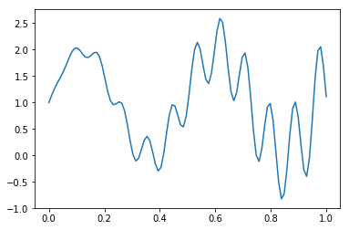
Integration
It is common to need to find areas under curves in statistics, for example, to estimate the probability mass under a distribution for a certain range of values.
In [68]:
d = stats.norm(0, 1)
In [69]:
integrate.quad(d.pdf, -1, 1)
Out[69]:
(0.682689492137086, 7.579375928402476e-15)
In [70]:
def f(x):
    return 1 + x * np.cos(71*x) + np.sin(13*x)
In [71]:
x = np.linspace(0, 1, 100)
plt.plot(x, f(x))
pass
In [72]:
integrate.quad(f, 0, 1)
Out[72]:
(1.020254939102394, 1.636375780468161e-14)
In [73]:
integrate.romberg(f, 0, 1)
Out[73]:
1.0202549391050357
In [74]:
integrate.trapz(f(x), x)
Out[74]:
1.0196541685543563
In [75]:
integrate.simps(f(x), x)
Out[75]:
1.0202546407742057
In [76]:
d = stats.multivariate_normal(np.zeros(2), np.eye(2))
In [77]:
integrate.nquad(lambda x, y: d.pdf([x, y]), [[-2,2], [-2,2]])
Out[77]:
(0.9110697462219217, 1.7566204076527952e-11)
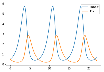
Integrating ODEs
In [78]:
def f(x, t, a, b, c, d):
    """Lotka-Volterra model."""
    u, v = x
    return [a*u + b*u*v, c*v + d*u*v]
In [79]:
a, b, c, d = 1, -1, -1, .5
x0 = [0.5,0.5]
t = np.linspace(0, 22, 100)
In [80]:
y = integrate.odeint(f, x0, t, args=(a,b,c,d))
plt.plot(t, y)
plt.legend(['rabbit','fox'], loc='best')
pass
Optimization
Scalar valued function
In [81]:
def f(x):
    return 3 + 4*x + 2*x**2
In [82]:
x = np.linspace(-4, 4, 100)
plt.plot(x, f(x))
pass
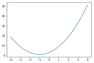
In [83]:
optimize.minimize_scalar(f)
Out[83]:
fun: 1.0
    nfev: 5
     nit: 4
 success: True
       x: -1.0000000000000002
In [84]:
x = np.linspace(-4, 4, 100)
plt.plot(x, np.cos(x))
pass
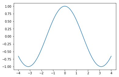
In [85]:
optimize.minimize_scalar(np.cos)
Out[85]:
fun: -1.0
    nfev: 9
     nit: 8
 success: True
       x: 3.1415926536439596
Provide bounds for bounded search
In [86]:
optimize.minimize_scalar(np.cos, bounds=[-2,0], method='bounded')
Out[86]:
fun: -0.41614319477908951
 message: 'Solution found.'
    nfev: 27
  status: 0
 success: True
       x: -1.9999959949686341
Provide brackets for downhill search
In [87]:
optimize.minimize_scalar(np.cos, bracket=[-1,-2])
Out[87]:
fun: -0.99999999999999989
    nfev: 8
     nit: 7
 success: True
       x: -3.1415926702696373
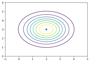
Vector-valued function
In [88]:
d = stats.multivariate_normal([2,3], np.eye(2))
In [89]:
x = np.linspace(-1,5,100)
y = np.linspace(0,6,100)
X, Y = np.meshgrid(x, y)
z = d.pdf(np.c_[X.ravel(), Y.ravel()]).reshape((100,100))
In [90]:
plt.contour(X, Y, z)
plt.scatter([[2]], [3])
pass
In [91]:
optimize.minimize(lambda x: -1*d.pdf(x), [0,0])
Out[91]:
fun: -0.15915494309093864
 hess_inv: array([[ 1212.355,  1817.032],
       [ 1817.032,  2726.548]])
      jac: array([  3.036e-07,   4.601e-07])
  message: 'Optimization terminated successfully.'
     nfev: 56
      nit: 2
     njev: 14
   status: 0
  success: True
        x: array([ 2.,  3.])
Constrained optimization
In [92]:
def f(x):
    return -(2*x[0]*x[1] + 2*x[0] - x[0]**2 - 2*x[1]**2)
In [93]:
x0 = [0, 2.5]
Unconstrained optimization
In [94]:
ux = optimize.minimize(f, x0, constraints=None)
ux
Out[94]:
fun: -1.9999999999996365
 hess_inv: array([[ 0.998,  0.501],
       [ 0.501,  0.499]])
      jac: array([  1.252e-06,  -1.416e-06])
  message: 'Optimization terminated successfully.'
     nfev: 24
      nit: 5
     njev: 6
   status: 0
  success: True
        x: array([ 2.,  1.])
Constrained optimization
In [95]:
cons = ({'type': 'eq',
         'fun' : lambda x: np.array([x[0]**3 - x[1]]),
         'jac' : lambda x: np.array([3.0*(x[0]**2.0), -1.0])},
        {'type': 'ineq',
         'fun' : lambda x: np.array([x[1] - (x[0]-1)**4 - 2])})

bnds = ((0.5, 1.5), (1.5, 2.5))
In [96]:
cx = optimize.minimize(f, x0, bounds=bnds, constraints=cons)
cx
Out[96]:
fun: 2.049915472092552
     jac: array([-3.487,  5.497])
 message: 'Optimization terminated successfully.'
    nfev: 21
     nit: 5
    njev: 5
  status: 0
 success: True
       x: array([ 1.261,  2.005])
In [97]:
x = np.linspace(0, 3, 100)
y = np.linspace(0, 3, 100)
X, Y = np.meshgrid(x, y)
Z = f(np.vstack([X.ravel(), Y.ravel()])).reshape((100,100))
plt.contour(X, Y, Z, np.arange(-1.99,10, 1));
plt.plot(x, x**3, 'k:', linewidth=1)
plt.plot(x, (x-1)**4+2, 'k:', linewidth=1)
plt.text(ux['x'][0], ux['x'][1], 'x', va='center', ha='center', size=20, color='blue')
plt.text(cx['x'][0], cx['x'][1], 'x', va='center', ha='center', size=20, color='red')
plt.fill([0.5,0.5,1.5,1.5], [2.5,1.5,1.5,2.5], alpha=0.3)
plt.axis([0,3,0,3]);

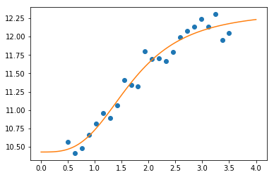
Curve-fitting
Curve fitting fits a scalar function to a series of data points. The
curve_fit method provides a convenient interface for curve fitting.
In [98]:
def logistic4(x, a, b, c, d):
    """The four paramter logistic function is often used to fit dose-response relationships."""
    return ((a-d)/(1.0+((x/c)**b))) + d
Generate some noisy observations
In [99]:
nobs = 24
xdata = np.linspace(0.5, 3.5, nobs)
ptrue = [10, 3, 1.5, 12]
ydata = logistic4(xdata, *ptrue) + 0.5*np.random.random(nobs)
In [100]:
popt, pcov = optimize.curve_fit(logistic4, xdata, ydata)
In [101]:
x = np.linspace(0, 4, 100)
y = logistic4(x, *popt)
plt.plot(xdata, ydata, 'o')
plt.plot(x, y)
pass
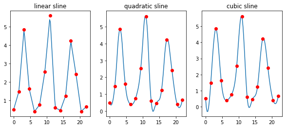
Interpolation
Interpolation constructs new data points given a set of known data points. Often, its objective is to estimate intermediate data points. Interpolation is most commonly done by fitting piecewise polynomials with certain constraints to make the join points continuous or smooth.
This is different from what we did with curve-fitting optimization, where we desire to approximate a complicated function with a simpler one.
In [102]:
def f(x, t, a, b, c, d):
    """Lotka-Volterra model."""
    u, v = x
    return [a*u + b*u*v, c*v + d*u*v]
In [103]:
t = np.linspace(0, 22, 15)
a, b, c, d = 1, -1, -1, .5
x0 = [0.5,0.5]
y = integrate.odeint(f, x0, t, args=(a,b,c,d))
In [104]:
rabbits = y[:, 0]
In [105]:
titles = ['linear', 'quadratic', 'cubic']
fig, axes = plt.subplots(1,3,figsize=(10, 4))

for i, ax in enumerate(axes, 1):
    ti = np.linspace(0, 22, 100)
    g = interpolate.interp1d(t, rabbits, kind=i)
    ax.plot(ti, g(ti))
    ax.plot(t, rabbits, 'ro')
    ax.set_title(titles[i-1] + ' sline')
pass
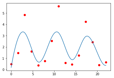
The default smooths quite heavily.
In [106]:
sp = interpolate.UnivariateSpline(t, rabbits)
plt.plot(t, rabbits, 'ro')
plt.plot(ti, sp(ti))
pass
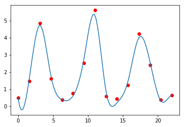
We can control the amount of smoothing.
In [107]:
sp = interpolate.UnivariateSpline(t, rabbits)
sp.set_smoothing_factor(0.5)
plt.plot(t, rabbits, 'ro')
plt.plot(ti, sp(ti))
pass
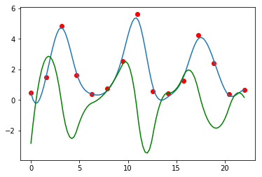
Finding derivatives.
In [108]:
sp = interpolate.UnivariateSpline(t, rabbits)
sp.set_smoothing_factor(0.5)
sp1 = sp.derivative()
plt.plot(t, rabbits, 'ro')
plt.plot(ti, sp(ti))
plt.plot(ti, sp1(ti), 'g')
pass
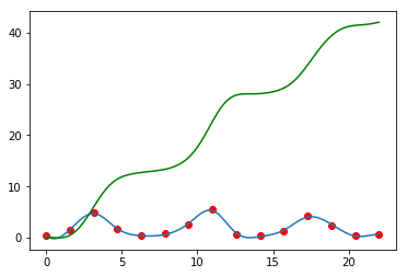
Finding integrals (AUC).
In [109]:
sp = interpolate.UnivariateSpline(t, rabbits)
sp.set_smoothing_factor(0.5)
sp2 = sp.antiderivative()
plt.plot(t, rabbits, 'ro')
plt.plot(ti, sp(ti))
plt.plot(ti, sp2(ti), 'g')
pass
Exercises
Exercise 1
If twice the age of son is added to age of father, the sum is 56. But if
twice the age of the father is added to the age of son, the sum is 82.
Find the ages of father and son. Do this using solve.
In [110]:
A = np.array([[2,1], [1,2]])
y = np.array([56, 82])
linalg.solve(A, y)
Out[110]:
array([ 10., 36.])
Exercise 2
Using the x and y data given below, estimate the parameters
a, b and c using lstsq() to fit a quadratic function.
Hints:
- The quadratic function is linear in the coefficients if you treat
xandx**2as observed constants. - The intercept can be found using a dummy variable which is always set to 1
- You will need to construct an \(N \times 3\) matrix to pass to
lstsq().
For each \(x_i\) and \(y_i\), we have
and this is equivalent to
suggests re-writing in matrix notation
where
In [111]:
n = 1000
a, b, c = 1, 2, 3
x = np.arange(n)
y = a + b*x + c*x**2 + np.random.normal(0, 1, n)
In [112]:
X = np.c_[np.ones(n), x, x**2]
linalg.lstsq(X, y)[0]
Out[112]:
array([ 1.003, 2. , 3. ])
Exercise 3
Estimate the probability of being between 0 and 3 for the PDF given below by integration.
In [113]:
from mystery import pdf
In [114]:
x = np.linspace(-3, 5, 100)
plt.plot(x, pdf(x))
pass
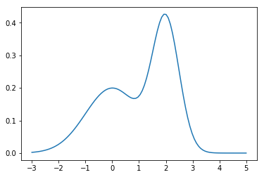
In [115]:
integrate.quad(pdf, 0, 3)
Out[115]:
(0.7379341493891789, 8.1927148211271e-15)
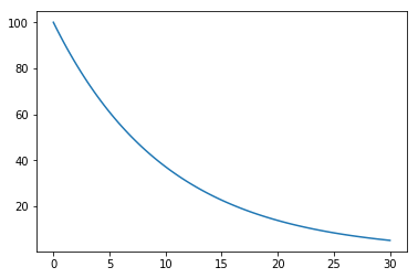
Exercise 4
Plot the amount of a radioactive substance over 30 days, if we start with 100 units and its half-life is 7 days.
In [116]:
def decay(x, t, mu):
    """dy/dt"""
    return -mu*x
In [117]:
x0 = 100
mu = np.log(2)/7
t = np.linspace(0, 30, 100)
y = integrate.odeint(decay, x0, t, args=(mu,))
plt.plot(t, y)
pass
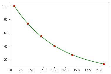
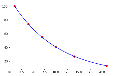
Exercise 5
You have some noisy measurements of the amount of radioactive material over time.
- Estimate the decay constant using the closed form solution for exponential decay
- Plot the observed data points in red
- Plot a fitted a decay curve in blue
- Plot a smooth interpolated curve using cubic splines in green
Recall the closed form solution
In [118]:
def f(t, x0, mu):
    return -mu*x0
In [119]:
t = np.array([1, 4, 7, 10, 14, 21])
y = np.array([ 100. , 74.082,  54.881, 40.657, 27.253, 13.534])
In [120]:
def orbit(t, x0, mu):
    """Closed form solution."""
    return x0 * np.exp(-mu * t)
In [121]:
popt, pcov = optimize.curve_fit(orbit, t, y)
x0, mu = popt
In [122]:
mu
Out[122]:
0.099999864435514327
In [123]:
plt.scatter(t, y, c='red')
tp = np.linspace(t[0], t[-1], 100)
yp = orbit(tp, x0, mu)
plt.plot(tp, yp, c='blue')
pass
In [124]:
plt.scatter(t, y, c='red')
f = interpolate.interp1d(t, y, kind='cubic')
plt.plot(tp, f(tp), c='green')
pass