Using optimization routines from scipy and statsmodels
In [1]:
%matplotlib inline
In [2]:
import scipy.linalg as la
import numpy as np
import scipy.optimize as opt
import matplotlib.pyplot as plt
import pandas as pd
In [3]:
np.set_printoptions(precision=3, suppress=True)
Using scipy.optimize
One of the most convenient libraries to use is scipy.optimize, since
it is already part of the Anaconda installation and it has a fairly
intuitive interface.
In [4]:
from scipy import optimize as opt
Minimizing a univariate function f:R→R
In [5]:
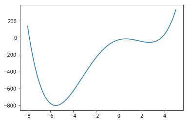
def f(x):
    return x**4 + 3*(x-2)**3 - 15*(x)**2 + 1
In [6]:
x = np.linspace(-8, 5, 100)
plt.plot(x, f(x));
The
`minimize_scalar <http://docs.scipy.org/doc/scipy/reference/generated/scipy.optimize.minimize_scalar.html#scipy.optimize.minimize_scalar>`__
function will find the minimum, and can also be told to search within
given bounds. By default, it uses the Brent algorithm, which combines a
bracketing strategy with a parabolic approximation.
In [7]:
opt.minimize_scalar(f, method='Brent')
Out[7]:
     fun: -803.3955308825884
    nfev: 12
     nit: 11
 success: True
       x: -5.528801125219663
In [8]:
opt.minimize_scalar(f, method='bounded', bounds=[0, 6])
Out[8]:
     fun: -54.21003937712762
 message: 'Solution found.'
    nfev: 12
  status: 0
 success: True
       x: 2.668865104039653
Local and global minima
In [9]:
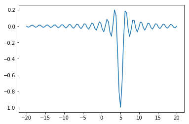
def f(x, offset):
    return -np.sinc(x-offset)
In [10]:
x = np.linspace(-20, 20, 100)
plt.plot(x, f(x, 5));
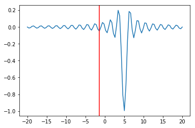
In [11]:
# note how additional function arguments are passed in
sol = opt.minimize_scalar(f, args=(5,))
sol
Out[11]:
     fun: -0.049029624014074166
    nfev: 11
     nit: 10
 success: True
       x: -1.4843871263953001
In [12]:
plt.plot(x, f(x, 5))
plt.axvline(sol.x, c='red')
pass
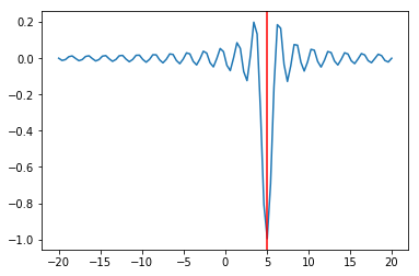
We can try multiple random starts to find the global minimum
In [13]:
lower = np.random.uniform(-20, 20, 100)
upper = lower + 1
sols = [opt.minimize_scalar(f, args=(5,), bracket=(l, u)) for (l, u) in zip(lower, upper)]
In [14]:
idx = np.argmin([sol.fun for sol in sols])
sol = sols[idx]
In [15]:
plt.plot(x, f(x, 5))
plt.axvline(sol.x, c='red');

Using a stochastic algorithm
See documentation for the
`basinhopping <http://docs.scipy.org/doc/scipy-0.14.0/reference/generated/scipy.optimize.basinhopping.html>`__
algorithm, which also works with multivariate scalar optimization. Note
that this is heuristic and not guaranteed to find a global minimum.
In [16]:
from scipy.optimize import basinhopping

x0 = 0
sol = basinhopping(f, x0, stepsize=1, minimizer_kwargs={'args': (5,)})
sol
Out[16]:
                        fun: -1.0
 lowest_optimization_result:       fun: -1.0
 hess_inv: array([[0.304]])
      jac: array([0.])
  message: 'Optimization terminated successfully.'
     nfev: 18
      nit: 4
     njev: 6
   status: 0
  success: True
        x: array([5.])
                    message: ['requested number of basinhopping iterations completed successfully']
      minimization_failures: 0
                       nfev: 1797
                        nit: 100
                       njev: 599
                          x: array([5.])
In [17]:
plt.plot(x, f(x, 5))
plt.axvline(sol.x, c='red');
Constrained optimization with scipy.optimize
Many real-world optimization problems have constraints - for example, a set of parameters may have to sum to 1.0 (equality constraint), or some parameters may have to be non-negative (inequality constraint). Sometimes, the constraints can be incorporated into the function to be minimized, for example, the non-negativity constraint p>0 can be removed by substituting p=eq and optimizing for q. Using such workarounds, it may be possible to convert a constrained optimization problem into an unconstrained one, and use the methods discussed above to solve the problem.
Alternatively, we can use optimization methods that allow the specification of constraints directly in the problem statement as shown in this section. Internally, constraint violation penalties, barriers and Lagrange multipliers are some of the methods used used to handle these constraints. We use the example provided in the Scipy tutorial to illustrate how to set constraints.
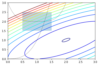
We will optimize:
In [18]:
def f(x):
    return -(2*x[0]*x[1] + 2*x[0] - x[0]**2 - 2*x[1]**2)
In [19]:
x = np.linspace(0, 3, 100)
y = np.linspace(0, 3, 100)
X, Y = np.meshgrid(x, y)
Z = f(np.vstack([X.ravel(), Y.ravel()])).reshape((100,100))
plt.contour(X, Y, Z, np.arange(-1.99,10, 1), cmap='jet');
plt.plot(x, x**3, 'k:', linewidth=1)
plt.plot(x, (x-1)**4+2, 'k:', linewidth=1)
plt.fill([0.5,0.5,1.5,1.5], [2.5,1.5,1.5,2.5], alpha=0.3)
plt.axis([0,3,0,3])
Out[19]:
[0, 3, 0, 3]
To set constraints, we pass in a dictionary with keys type, fun
and jac. Note that the inequality constraint assumes a
Cjx≥0 form. As usual, the jac is optional and will be
numerically estimated if not provided.
In [20]:
cons = ({'type': 'eq',
         'fun' : lambda x: np.array([x[0]**3 - x[1]]),
         'jac' : lambda x: np.array([3.0*(x[0]**2.0), -1.0])},
        {'type': 'ineq',
         'fun' : lambda x: np.array([x[1] - (x[0]-1)**4 - 2])})

bnds = ((0.5, 1.5), (1.5, 2.5))
In [21]:
x0 = [0, 2.5]
Unconstrained optimization
In [22]:
ux = opt.minimize(f, x0, constraints=None)
ux
Out[22]:
      fun: -1.9999999999996365
 hess_inv: array([[0.998, 0.501],
       [0.501, 0.499]])
      jac: array([ 0., -0.])
  message: 'Optimization terminated successfully.'
     nfev: 24
      nit: 5
     njev: 6
   status: 0
  success: True
        x: array([2., 1.])
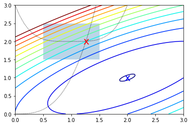
Constrained optimization
In [23]:
cx = opt.minimize(f, x0, bounds=bnds, constraints=cons)
cx
Out[23]:
     fun: 2.049915472024102
     jac: array([-3.487,  5.497])
 message: 'Optimization terminated successfully.'
    nfev: 25
     nit: 6
    njev: 6
  status: 0
 success: True
       x: array([1.261, 2.005])
In [24]:
x = np.linspace(0, 3, 100)
y = np.linspace(0, 3, 100)
X, Y = np.meshgrid(x, y)
Z = f(np.vstack([X.ravel(), Y.ravel()])).reshape((100,100))
plt.contour(X, Y, Z, np.arange(-1.99,10, 1), cmap='jet');
plt.plot(x, x**3, 'k:', linewidth=1)
plt.plot(x, (x-1)**4+2, 'k:', linewidth=1)
plt.text(ux['x'][0], ux['x'][1], 'x', va='center', ha='center', size=20, color='blue')
plt.text(cx['x'][0], cx['x'][1], 'x', va='center', ha='center', size=20, color='red')
plt.fill([0.5,0.5,1.5,1.5], [2.5,1.5,1.5,2.5], alpha=0.3)
plt.axis([0,3,0,3]);
Some applications of optimization
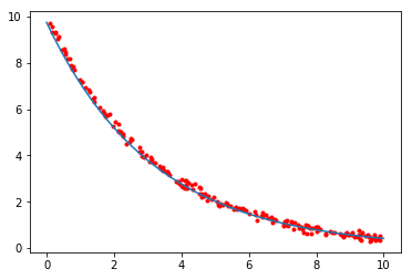
This is a specialized application of curve_fit, in which the curve
to be fitted is defined implicitly by an ordinary differential equation
and the initial value x0. Of course this can be explicitly solved but the same approach can be used to find multiple parameters for n-dimensional systems of ODEs.
A more elaborate example for fitting a system of ODEs to model the zombie apocalypse
In [25]:
from scipy.integrate import odeint

def f(x, t, k):
    """Simple exponential decay."""
    return -k*x

def x(t, k, x0):
    """
    Solution to the ODE x'(t) = f(t,x,k) with initial condition x(0) = x0
    """
    x = odeint(f, x0, t, args=(k,))
    return x.ravel()
In [26]:
# True parameter values
x0_ = 10
k_ = 0.1*np.pi

# Some random data genererated from closed form solution plus Gaussian noise
ts = np.sort(np.random.uniform(0, 10, 200))
xs = x0_*np.exp(-k_*ts) + np.random.normal(0,0.1,200)

popt, cov = opt.curve_fit(x, ts, xs)
k_opt, x0_opt = popt

print("k = %g" % k_opt)
print("x0 = %g" % x0_opt)
k = 0.314378
x0 = 9.74377
In [27]:
import matplotlib.pyplot as plt
t = np.linspace(0, 10, 100)
plt.plot(ts, xs, 'r.', t, x(t, k_opt, x0_opt), '-');
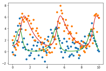
You may have to install the
`lmfit <http://cars9.uchicago.edu/software/python/lmfit/index.html>`__
package using pip and restart your kernel. The lmfit algorithm
is another wrapper around scipy.optimize.leastsq but allows for
richer model specification and more diagnostics.
In [28]:
! pip install lmfit
Requirement already satisfied: lmfit in /usr/local/lib/python3.6/site-packages (0.9.11)
Requirement already satisfied: scipy>=0.17 in /usr/local/lib/python3.6/site-packages (from lmfit) (1.0.1)
Requirement already satisfied: six>1.10 in /usr/local/lib/python3.6/site-packages (from lmfit) (1.11.0)
Requirement already satisfied: numpy>=1.10 in /usr/local/lib/python3.6/site-packages (from lmfit) (1.14.2)
Requirement already satisfied: asteval>=0.9.12 in /usr/local/lib/python3.6/site-packages (from lmfit) (0.9.13)
Requirement already satisfied: uncertainties>=3.0 in /usr/local/lib/python3.6/site-packages (from lmfit) (3.0.2)
You are using pip version 18.0, however version 18.1 is available.
You should consider upgrading via the 'pip install --upgrade pip' command.
In [29]:
from lmfit import minimize, Parameters, Parameter, report_fit
import warnings
In [30]:
def f(xs, t, ps):
    """Lotka-Volterra predator-prey model."""
    try:
        a = ps['a'].value
        b = ps['b'].value
        c = ps['c'].value
        d = ps['d'].value
    except:
        a, b, c, d = ps

    x, y = xs
    return [a*x - b*x*y, c*x*y - d*y]

def g(t, x0, ps):
    """
    Solution to the ODE x'(t) = f(t,x,k) with initial condition x(0) = x0
    """
    x = odeint(f, x0, t, args=(ps,))
    return x

def residual(ps, ts, data):
    x0 = ps['x0'].value, ps['y0'].value
    model = g(ts, x0, ps)
    return (model - data).ravel()

t = np.linspace(0, 10, 100)
x0 = np.array([1,1])

a, b, c, d = 3,1,1,1
true_params = np.array((a, b, c, d))

np.random.seed(123)
data = g(t, x0, true_params)
data += np.random.normal(size=data.shape)

# set parameters incluing bounds
params = Parameters()
params.add('x0', value= float(data[0, 0]), min=0, max=10)
params.add('y0', value=float(data[0, 1]), min=0, max=10)
params.add('a', value=2.0, min=0, max=10)
params.add('b', value=2.0, min=0, max=10)
params.add('c', value=2.0, min=0, max=10)
params.add('d', value=2.0, min=0, max=10)

# fit model and find predicted values
result = minimize(residual, params, args=(t, data), method='leastsq')
final = data + result.residual.reshape(data.shape)

# plot data and fitted curves
plt.plot(t, data, 'o')
plt.plot(t, final, '-', linewidth=2);

# display fitted statistics
report_fit(result)
[[Fit Statistics]]
    # fitting method   = leastsq
    # function evals   = 167
    # data points      = 200
    # variables        = 6
    chi-square         = 212.716019
    reduced chi-square = 1.09647432
    Akaike info crit   = 24.3281329
    Bayesian info crit = 44.1180371
[[Variables]]
    x0:  1.02052198 +/- 0.18168320 (17.80%) (init = 0)
    y0:  1.07046509 +/- 0.11017748 (10.29%) (init = 1.997345)
    a:   3.54341849 +/- 0.45416005 (12.82%) (init = 2)
    b:   1.21280681 +/- 0.14847542 (12.24%) (init = 2)
    c:   0.84529665 +/- 0.07947808 (9.40%) (init = 2)
    d:   0.85715536 +/- 0.08562777 (9.99%) (init = 2)
[[Correlations]] (unreported correlations are < 0.100)
    C(a, b)  =  0.960
    C(a, d)  = -0.956
    C(b, d)  = -0.878
    C(x0, b) = -0.759
    C(x0, a) = -0.745
    C(y0, c) = -0.717
    C(y0, d) = -0.683
    C(c, d)  =  0.667
    C(x0, d) =  0.578
    C(a, c)  = -0.532
    C(y0, a) =  0.475
    C(b, c)  = -0.433
    C(y0, b) =  0.271
Optimization of graph node placement
To show the many different applications of optimization, here is an example using optimization to change the layout of nodes of a graph. We use a physical analogy - nodes are connected by springs, and the springs resist deformation from their natural length lij. Some nodes are pinned to their initial locations while others are free to move. Because the initial configuration of nodes does not have springs at their natural length, there is tension resulting in a high potential energy U, given by the physics formula shown below. Optimization finds the configuration of lowest potential energy given that some nodes are fixed (set up as boundary constraints on the positions of the nodes).
Note that the ordination algorithm Multi-Dimensional Scaling (MDS) works on a very similar idea - take a high dimensional data set in Rn, and project down to a lower dimension (Rk) such that the sum of distances dn(xi,xj)−dk(xi,xj), where dn and dk are some measure of distance between two points xi and xj in n and d dimension respectively, is minimized. MDS is often used in exploratory analysis of high-dimensional data to get some intuitive understanding of its “structure”.
In [31]:
from scipy.spatial.distance import pdist, squareform
- P0 is the initial location of nodes
- P is the minimal energy location of nodes given constraints
- A is a connectivity matrix - there is a spring between i and j if Aij=1
- Lij is the resting length of the spring connecting i and j
- In addition, there are a number of
fixednodes whose positions are pinned.
In [32]:
n = 20
k = 1 # spring stiffness
P0 = np.random.uniform(0, 5, (n,2))
A = np.ones((n, n))
A[np.tril_indices_from(A)] = 0
L = A.copy()
In [33]:
L.astype('int')
Out[33]:
array([[0, 1, 1, 1, 1, 1, 1, 1, 1, 1, 1, 1, 1, 1, 1, 1, 1, 1, 1, 1],
       [0, 0, 1, 1, 1, 1, 1, 1, 1, 1, 1, 1, 1, 1, 1, 1, 1, 1, 1, 1],
       [0, 0, 0, 1, 1, 1, 1, 1, 1, 1, 1, 1, 1, 1, 1, 1, 1, 1, 1, 1],
       [0, 0, 0, 0, 1, 1, 1, 1, 1, 1, 1, 1, 1, 1, 1, 1, 1, 1, 1, 1],
       [0, 0, 0, 0, 0, 1, 1, 1, 1, 1, 1, 1, 1, 1, 1, 1, 1, 1, 1, 1],
       [0, 0, 0, 0, 0, 0, 1, 1, 1, 1, 1, 1, 1, 1, 1, 1, 1, 1, 1, 1],
       [0, 0, 0, 0, 0, 0, 0, 1, 1, 1, 1, 1, 1, 1, 1, 1, 1, 1, 1, 1],
       [0, 0, 0, 0, 0, 0, 0, 0, 1, 1, 1, 1, 1, 1, 1, 1, 1, 1, 1, 1],
       [0, 0, 0, 0, 0, 0, 0, 0, 0, 1, 1, 1, 1, 1, 1, 1, 1, 1, 1, 1],
       [0, 0, 0, 0, 0, 0, 0, 0, 0, 0, 1, 1, 1, 1, 1, 1, 1, 1, 1, 1],
       [0, 0, 0, 0, 0, 0, 0, 0, 0, 0, 0, 1, 1, 1, 1, 1, 1, 1, 1, 1],
       [0, 0, 0, 0, 0, 0, 0, 0, 0, 0, 0, 0, 1, 1, 1, 1, 1, 1, 1, 1],
       [0, 0, 0, 0, 0, 0, 0, 0, 0, 0, 0, 0, 0, 1, 1, 1, 1, 1, 1, 1],
       [0, 0, 0, 0, 0, 0, 0, 0, 0, 0, 0, 0, 0, 0, 1, 1, 1, 1, 1, 1],
       [0, 0, 0, 0, 0, 0, 0, 0, 0, 0, 0, 0, 0, 0, 0, 1, 1, 1, 1, 1],
       [0, 0, 0, 0, 0, 0, 0, 0, 0, 0, 0, 0, 0, 0, 0, 0, 1, 1, 1, 1],
       [0, 0, 0, 0, 0, 0, 0, 0, 0, 0, 0, 0, 0, 0, 0, 0, 0, 1, 1, 1],
       [0, 0, 0, 0, 0, 0, 0, 0, 0, 0, 0, 0, 0, 0, 0, 0, 0, 0, 1, 1],
       [0, 0, 0, 0, 0, 0, 0, 0, 0, 0, 0, 0, 0, 0, 0, 0, 0, 0, 0, 1],
       [0, 0, 0, 0, 0, 0, 0, 0, 0, 0, 0, 0, 0, 0, 0, 0, 0, 0, 0, 0]])
In [34]:
def energy(P):
    P = P.reshape((-1, 2))
    D = squareform(pdist(P))
    return 0.5*(k * A * (D - L)**2).sum()
In [35]:
D0 = squareform(pdist(P0))
E0 = 0.5* k * A * (D0 - L)**2
In [36]:
D0[:5, :5]
Out[36]:
array([[0.   , 5.039, 0.921, 1.758, 1.99 ],
       [5.039, 0.   , 5.546, 3.414, 4.965],
       [0.921, 5.546, 0.   , 2.133, 2.888],
       [1.758, 3.414, 2.133, 0.   , 2.762],
       [1.99 , 4.965, 2.888, 2.762, 0.   ]])
In [37]:
E0[:5, :5]
Out[37]:
array([[ 0.   ,  8.159,  0.003,  0.288,  0.49 ],
       [ 0.   ,  0.   , 10.333,  2.915,  7.862],
       [ 0.   ,  0.   ,  0.   ,  0.642,  1.782],
       [ 0.   ,  0.   ,  0.   ,  0.   ,  1.552],
       [ 0.   ,  0.   ,  0.   ,  0.   ,  0.   ]])
In [38]:
energy(P0.ravel())
Out[38]:
479.13650839857024
In [39]:
# fix the position of the first few nodes just to show constraints
fixed = 4
bounds = (np.repeat(P0[:fixed,:].ravel(), 2).reshape((-1,2)).tolist() +
          [[None, None]] * (2*(n-fixed)))
In [40]:
P0[:5]
Out[40]:
array([[1.191, 4.039],
       [4.475, 0.216],
       [1.51 , 4.903],
       [2.698, 3.132],
       [0.028, 2.425]])
In [41]:
bounds[:10]
Out[41]:
[[1.191249528562059, 1.191249528562059],
 [4.0389554314507805, 4.0389554314507805],
 [4.474891439430058, 4.474891439430058],
 [0.216114460398234, 0.216114460398234],
 [1.5097341813135952, 1.5097341813135952],
 [4.902910992971438, 4.902910992971438],
 [2.6975241127686767, 2.6975241127686767],
 [3.1315468085492815, 3.1315468085492815],
 [None, None],
 [None, None]]
In [42]:
sol = opt.minimize(energy, P0.ravel(), bounds=bounds)
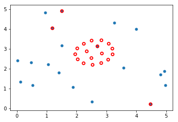
Visualization
Original placement is BLUE Optimized arrangement is RED.
In [43]:
plt.scatter(P0[:, 0], P0[:, 1], s=25)
P = sol.x.reshape((-1,2))
plt.scatter(P[:, 0], P[:, 1], edgecolors='red', facecolors='none', s=30, linewidth=2);
Optimization of standard statistical models
When we solve standard statistical problems, an optimization procedure similar to the ones discussed here is performed. For example, consider multivariate logistic regression - typically, a Newton-like algorithm known as iteratively reweighted least squares (IRLS) is used to find the maximum likelihood estimate for the generalized linear model family. However, using one of the multivariate scalar minimization methods shown above will also work, for example, the BFGS minimization algorithm.
The take home message is that there is nothing magic going on when Python or R fits a statistical model using a formula - all that is happening is that the objective function is set to be the negative of the log likelihood, and the minimum found using some first or second order optimization algorithm.
In [44]:
import statsmodels.api as sm
Suppose we have a binary outcome measure Y∈0,1 that is conditinal on some input variable (vector) x∈(−∞,+∞). Let the conditioanl probability be p(x)=P(Y=y|X=x). Given some data, one simple probability model is p(x)=β0+x⋅β - i.e. linear regression. This doesn’t really work for the obvious reason that p(x) must be between 0 and 1 as x ranges across the real line. One simple way to fix this is to use the transformation g(x)=p(x)1−p(x)=β0+x.β. Solving for p, we get
Suppose we have n data points (xi,yi) where xi is a vector of features and yi is an observed class (0 or 1). For each event, we either have “success” (y=1) or “failure” (Y=0), so the likelihood looks like the product of Bernoulli random variables. According to the logistic model, the probability of success is p(xi) if yi=1 and 1−p(xi) if yi=0. So the likelihood is
Using the standard ‘trick’, if we augment the matrix X with a column of 1s, we can write β0+xi⋅β as just Xβ.
In [45]:
df_ = pd.read_csv("https://stats.idre.ucla.edu/stat/data/binary.csv")
df_.head()
Out[45]:
| admit | gre | gpa | rank | |
|---|---|---|---|---|
| 0 | 0 | 380 | 3.61 | 3 |
| 1 | 1 | 660 | 3.67 | 3 |
| 2 | 1 | 800 | 4.00 | 1 |
| 3 | 1 | 640 | 3.19 | 4 |
| 4 | 0 | 520 | 2.93 | 4 |
In [46]:
# We will ignore the rank categorical value

cols_to_keep = ['admit', 'gre', 'gpa']
df = df_[cols_to_keep]
df.insert(1, 'dummy', 1)
df.head()
Out[46]:
| admit | dummy | gre | gpa | |
|---|---|---|---|---|
| 0 | 0 | 1 | 380 | 3.61 |
| 1 | 1 | 1 | 660 | 3.67 |
| 2 | 1 | 1 | 800 | 4.00 |
| 3 | 1 | 1 | 640 | 3.19 |
| 4 | 0 | 1 | 520 | 2.93 |
This is very similar to what you would do in R, only using Python’s
statsmodels package. The GLM solver uses a special variant of
Newton’s method known as iteratively reweighted least squares (IRLS),
which will be further desribed in the lecture on multivarite and
constrained optimizaiton.
In [47]:
model = sm.GLM.from_formula('admit ~ gre + gpa',
                            data=df, family=sm.families.Binomial())
fit = model.fit()
fit.summary()
Out[47]:
| Dep. Variable: | admit | No. Observations: | 400 |
|---|---|---|---|
| Model: | GLM | Df Residuals: | 397 |
| Model Family: | Binomial | Df Model: | 2 |
| Link Function: | logit | Scale: | 1.0000 |
| Method: | IRLS | Log-Likelihood: | -240.17 |
| Date: | Mon, 15 Oct 2018 | Deviance: | 480.34 |
| Time: | 16:04:00 | Pearson chi2: | 398. |
| No. Iterations: | 4 | Covariance Type: | nonrobust |
| coef | std err | z | P>|z| | [0.025 | 0.975] | |
|---|---|---|---|---|---|---|
| Intercept | -4.9494 | 1.075 | -4.604 | 0.000 | -7.057 | -2.842 |
| gre | 0.0027 | 0.001 | 2.544 | 0.011 | 0.001 | 0.005 |
| gpa | 0.7547 | 0.320 | 2.361 | 0.018 | 0.128 | 1.381 |
In [48]:
%load_ext rpy2.ipython
In [49]:
%%R -i df
m <- glm(admit ~ gre + gpa, data=df, family="binomial")
summary(m)
Call:
glm(formula = admit ~ gre + gpa, family = "binomial", data = df)

Deviance Residuals:
    Min       1Q   Median       3Q      Max
-1.2730  -0.8988  -0.7206   1.3013   2.0620

Coefficients:
             Estimate Std. Error z value Pr(>|z|)
(Intercept) -4.949378   1.075093  -4.604 4.15e-06 ***
gre          0.002691   0.001057   2.544   0.0109 *
gpa          0.754687   0.319586   2.361   0.0182 *
---
Signif. codes:  0 ‘***’ 0.001 ‘**’ 0.01 ‘*’ 0.05 ‘.’ 0.1 ‘ ’ 1

(Dispersion parameter for binomial family taken to be 1)

    Null deviance: 499.98  on 399  degrees of freedom
Residual deviance: 480.34  on 397  degrees of freedom
AIC: 486.34

Number of Fisher Scoring iterations: 4
This is to show that there is no magic going on - you can write the function to minimize directly from the log-likelihood equation and run a minimizer. It will be more accurate if you also provide the derivative (+/- the Hessian for second order methods), but using just the function and numerical approximations to the derivative will also work. As usual, this is for illustration so you understand what is going on - when there is a library function available, you should probably use that instead.
In [50]:
def f(beta, y, x):
    """Minus log likelihood function for logistic regression."""
    return -((-np.log(1 + np.exp(np.dot(x, beta)))).sum() + (y*(np.dot(x, beta))).sum())
In [51]:
beta0 = np.zeros(3)
opt.minimize(f, beta0, args=(df['admit'], df.loc[:, 'dummy':]),
             method='BFGS', options={'gtol':1e-2})
Out[51]:
      fun: 240.17199087225998
 hess_inv: array([[ 1.122, -0.   , -0.271],
       [-0.   ,  0.   , -0.   ],
       [-0.271, -0.   ,  0.098]])
      jac: array([-0.   , -0.002, -0.   ])
  message: 'Optimization terminated successfully.'
     nfev: 65
      nit: 8
     njev: 13
   status: 0
  success: True
        x: array([-4.949,  0.003,  0.755])
There are also many optimization routines in the scikit-learn
package, as you already know from the previous lectures. Many machine
learning problems essentially boil down to the minimization of some
appropriate loss function.