Solving Optimization Problems Computationally

%matplotlib inline
%load_ext rpy2.ipython

import os
import glob
from pathlib import Path
import numpy as np
import pandas as pd
import matplotlib as mpl
import matplotlib.pyplot as plt
import seaborn as sns

sns.set_context('notebook', font_scale=1.5)

import scipy.linalg as la
import scipy.optimize as opt

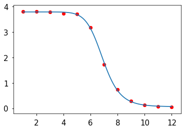
1. Curve fitting

Actual data from an ELISA experiment. The first column is log concentration, the second is the measured value from the ELISA assay at that concentration. Our task is to fit a 4 parameter logistic function to the observed data.

The 4 parameter logistic has the following form

\[f(x) = \frac{A-D}{1+(x/C)^B}+ D\]

where \(A\), \(B\), \(C\) and \(D\) are parameters to be determined.

Inspect data

data = np.array(
    [[ 1.   ,  3.802],
     [ 2.   ,  3.802],
     [ 3.   ,  3.778],
     [ 4.   ,  3.718],
     [ 5.   ,  3.696],
     [ 6.   ,  3.181],
     [ 7.   ,  1.731],
     [ 8.   ,  0.744],
     [ 9.   ,  0.29 ],
     [10.   ,  0.124],
     [11.   ,  0.064],
     [12.   ,  0.05 ]]
)

x = data[:, 0]
y = data[:, 1]

plt.scatter(x, y, c='red')
pass

Define 4 parameter logistic

def f(x, A, B, C, D):
    return (A - D)/(1 + (x/C)**B)  + D

Find reasonable values for initial parameters

A0 = y.max()
D0 = y.min()
C0 = x.mean()
B0 = 1
p0 = [A0, B0, C0, D0]

Using minimize with conjugate-gradient

Define the loss function

def loss(p, y, x):
    A, B, C, D = p
    return np.sum((y - f(x, A, B, C, D))**2)

Minimize

r = opt.minimize(loss, p0, args=(y, x), method='CG')

r.x

array([ 3.78699634, 10.87666589,  6.91225087,  0.06131771])

Plot the fit

xp = np.linspace(x.min(), x.max(), 100)
plt.plot(xp, f(xp, *r.x))
plt.scatter(x, y, c='red')
pass

Using nonlinear least squares

Define least squares residues

def res(p, y, x):
    A, B, C, D = p
    return (y - f(x, A, B, C, D))**2

Minimize

r = opt.least_squares(res, p0, args=(y, x))

r.x

array([ 3.7756568 , 11.02097427,  6.90573049,  0.07695251])

Plot

xp = np.linspace(x.min(), x.max(), 100)
plt.plot(xp, f(xp, *r.x))
plt.scatter(x, y, c='red')
pass

Using curve_fit

This is the most convenient as you can work with the function directly. It uses the Levenberg-Marquadt algorithm.

Minimize

p, pcov = opt.curve_fit(f, x, y, p0)

p

array([ 3.78699349, 10.87690577,  6.91224723,  0.06132645])

Plot

xp = np.linspace(x.min(), x.max(), 100)
plt.plot(xp, f(xp, *p))
plt.scatter(x, y, c='red')
pass

2. Constrained optimization

A. Using scipy.optimize, find the values of \(x\) and \(y\) that minimize \(e^{x^2 + y^2}\) in the unconstrained case and in the presence of the constraint that \(x + y = 3\). Use (1,1) as a starting guess.

opt.minimize(lambda x: np.exp(x[0]**2 + x[1]**2),
            np.ones(2))

      fun: 1.0000000000000002
 hess_inv: array([[ 0.74999784, -0.25000216],
       [-0.25000216,  0.74999784]])
      jac: array([0., 0.])
  message: 'Optimization terminated successfully.'
     nfev: 32
      nit: 7
     njev: 8
   status: 0
  success: True
        x: array([-8.0369005e-09, -8.0369005e-09])

opt.minimize(lambda x: np.exp(x[0]**2 + x[1]**2),
             np.ones(2),
             constraints=dict(type='eq', fun=lambda x: x[0] + x[1] - 3))

     fun: 90.01713130056051
     jac: array([270.05131435, 270.05148602])
 message: 'Optimization terminated successfully.'
    nfev: 44
     nit: 9
    njev: 9
  status: 0
 success: True
       x: array([1.49999954, 1.50000046])

B. A milkmaid is at point A and needs to get to point B. However, she also needs to fill a pail of water from the river en route from A to B. The equation of the river’s path is shown in the figure below. What is the minimum distance she has to travel to do this?

Milkmaid problem

def f(x, A, B):
    return la.norm(x-A) + la.norm(x-B)

def g(x):
    return x[1] - 10.0/(1 + x[0])

The solution is sensitive to the starting conditions.

x0 = np.array([4, 2])
A = np.array([2,8])
B = np.array([8,4])
cons = {'type': 'eq', 'fun': g}

res = opt.minimize(f, x0, args=(A, B), constraints=cons)
res.x, res.fun

(array([4.39881339, 1.85225887]), 10.792179122216428)

xp = np.linspace(0, 10, 100)
plt.scatter([A[0], B[0]], [A[1], B[1]])
plt.plot(xp, 10.0/(1 + xp), c='blue')
plt.plot([A[0], res.x[0], B[0]], [A[1], res.x[1], B[1]], c='red')
pass

We know that solutions must be along the river, so start with equally spaced points (in the x-direction) along the river.

x0s = [(x, 10/(1+x)) for x in range(11)]

best_x = None
best_fun = np.infty

A = np.array([2,8])
B = np.array([8,4])
cons = {'type': 'eq', 'fun': g}

for x0 in x0s:
    res = opt.minimize(f, x0, args=(A, B), constraints=cons)
    x, fun = res.x, res.fun
    if fun < best_fun:
        best_fun = fun
        best_x = x

best_x, best_fun

(array([0.53225961, 6.52630922]), 9.96339829956226)

xp = np.linspace(0, 10, 100)
plt.scatter([A[0], B[0]], [A[1], B[1]])
plt.plot(xp, 10.0/(1 + xp), c='blue')
plt.plot([A[0], best_x[0], B[0]], [A[1], best_x[1], B[1]], c='red')
pass

C. Find the minimum of the following quadratic function on \(\mathbb{R}^2\)

\[ \begin{align}\begin{aligned}f(x) = x^TAx +b^Tx +c\\where\end{aligned}\end{align} \]

\[\begin{split}A = \left(\begin{matrix}13&5\\5&7\end{matrix}\right), b = \left(\begin{matrix}1\\1\end{matrix}\right) \textrm {and } c = 2\end{split}\]

Under the constraints:

\[g(x) = 2x_1-5x_2=2 \;\;\;\;\;\; \textrm{ and } \;\;\;\;\;\; h(x) = x_1+x_2=1\]

1. Use a matrix decomposition method to find the minimum of the unconstrained problem without using scipy.optimize (Use library functions - no need to code your own). Note: for full credit you should exploit matrix structure. (3 points)
2. Find the solution using constrained optimization with the scipy.optimize package. (3 points)
3. Use Lagrange multipliers and solving the resulting set of equations directly without using scipy.optimize. (4 points)

A = np.array([[13,5],[5,7]])
b = np.array([1.0,1.0]).T
c = 2

la.cho_solve(la.cho_factor(A), -b/2)

array([-0.01515152, -0.06060606])

def f(x, A, b, c):
    return x.T.dot(A).dot(x) + b.T.dot(x) + c

# check unconstrained solution
usol = opt.minimize(f, [0,0], args=(A, b, c))
usol.x

array([-0.01515152, -0.06060606])

cons = ({'type': 'eq', 'fun': lambda x: 2*x[0] - 5*x[1] - 2},
        {'type': 'eq', 'fun': lambda x: x[0] + x[1] - 1})

opt.minimize(f, [0,0], constraints=cons, args=(A, b, c))

     fun: 15.999999999999996
     jac: array([26.99999976, 11.00000024])
 message: 'Optimization terminated successfully.'
    nfev: 14
     nit: 3
    njev: 3
  status: 0
 success: True
       x: array([1.00000000e+00, 3.41607086e-16])

M = np.array([
    [26, 10, 2, 1],
    [10, 14, -5, 1],
    [2, -5, 0, 0],
    [1, 1, 0, 0]
])

y = np.array([-1, -1, 2, 1]).T

la.solve(M, y)

array([ 1.00000000e+00, -4.37360585e-17, -2.28571429e+00, -2.24285714e+01])

3. Gradient descent

We observe some data points \((x_i, y_i)\), and believe that an appropriate model for the data is that

\[f(x) = ax^2 + bx^3 + c\sin{x}\]

with some added noise. Find optimal values of the parameters \(\beta = (a, b, c)\) that minimize \(\Vert y - f(x) \Vert^2\)

1. using scipy.linalg.lstsq (10 points)
2. solving the normal equations \(X^TX \beta = X^Ty\) (10 points)
3. using scipy.linalg.svd (10 points)
4. using gradient descent with RMSProp (no bias correction) and starting with an initial value of \(\beta = \begin{bmatrix}1 & 1 & 1\end{bmatrix}\). Use a learning rate of 0.01 and 10,000 iterations. This should take a few seconds to complete. (25 points)

In each case, plot the data and fitted curve using matplotlib.

Data

x = array([ 3.4027718 ,  4.29209002,  5.88176277,  6.3465969 ,  7.21397852,
        8.26972154, 10.27244608, 10.44703778, 10.79203455, 14.71146298])
y = array([ 25.54026428,  29.4558919 ,  58.50315846,  70.24957254,
        90.55155435, 100.56372833,  91.83189927,  90.41536733,
        90.43103028,  23.0719842 ])

x = np.array([ 3.4027718 ,  4.29209002,  5.88176277,  6.3465969 ,  7.21397852,
        8.26972154, 10.27244608, 10.44703778, 10.79203455, 14.71146298])
y = np.array([ 25.54026428,  29.4558919 ,  58.50315846,  70.24957254,
        90.55155435, 100.56372833,  91.83189927,  90.41536733,
        90.43103028,  23.0719842 ])

def f(beta, x):
    """Model function."""

    return beta[0]*x**2 + beta[1]*x**3 + beta[2]*np.sin(x)

X = np.c_[x**2, x**3, np.sin(x)]

Least squares solution

beta = np.linalg.lstsq(X, y, rcond=None)[0]

beta

array([ 2.99259014, -0.19883227, 10.20024689])

plt.plot(x, y, 'o')
xp = np.linspace(0, 15, 100)
plt.plot(xp, f(beta, xp))
pass

Normal equations solution

beta = np.linalg.solve(X.T @ X, X.T @ y)
beta

array([ 2.99259014, -0.19883227, 10.20024689])

plt.plot(x, y, 'o')
xp = np.linspace(0, 15, 100)
plt.plot(xp, f(beta, xp))
pass

SVD solution

U, s, Vt = np.linalg.svd(X)
beta = Vt.T @ np.diag(1/s) @ U[:, :len(s)].T @ y.reshape(-1,1)
beta

array([[ 2.99259014],
       [-0.19883227],
       [10.20024689]])

plt.plot(x, y, 'o')
xp = np.linspace(0, 15, 100)
plt.plot(xp, f(beta, xp))
pass

Gradient descent solution (with ADAM)

def res(beta, x, y):
    """Resdiual funciton."""
    return f(beta, x) - y

Scalar form for gradient

def grad(beta, x, y):
    """Gradient of function."""

    return np.array([
        np.sum(x**2 * res(beta, x, y)),
        np.sum(x**3 * res(beta, x, y)),
        np.sum(np.sin(x) * res(beta, x, y))
    ])

def gd(beta, x, y, f, grad, alpha=0.01, beta1=0.9, beta2=0.999, eps=1e-8):
    """Gradient descent."""

    m = 0
    v = 0
    for i in range(10000):
        m = beta1*m + (1-beta1)*grad(beta, x, y)
        v = beta2*v + (1-beta2)*grad(beta, x, y)**2
        mc = m/(1+beta1**(i+1))
        vc = v/(1+beta2**(i+1))
        beta = beta - alpha * m / (eps + np.sqrt(vc))
    return beta

beta = gd(np.array([1,1,1]), x, y, f, grad)
beta

array([ 2.99259014, -0.19883227, 10.20024689])

plt.plot(x, y, 'o')
xp = np.linspace(0, 15, 100)
plt.plot(xp, f(beta, xp))
pass

Matrix form for gradient

def grad_m(X, y, b):
    return X.T@X@b - X.T@y

Check that both gradient functions give the same solution

grad(np.zeros(3), x, y)

array([-5.23658157e+04, -5.13828104e+05,  1.02460119e+02])

X = np.c_[x**2, x**3, np.sin(x)]
grad_m(X, y, np.zeros(3))

array([-5.23658157e+04, -5.13828104e+05,  1.02460119e+02])

def gd_m(beta, x, y, f, grad, alpha=0.01, beta1=0.9, beta2=0.999, eps=1e-8):
    """Gradient descent."""

    m = 0
    v = 0
    X = np.c_[x**2, x**3, np.sin(x)]

    for i in range(10000):
        m = beta1*m + (1-beta1)*grad_m(X, y, beta)
        v = beta2*v + (1-beta2)*grad_m(X, y, beta)**2
        mc = m/(1+beta1**(i+1))
        vc = v/(1+beta2**(i+1))
        beta = beta - alpha * m / (eps + np.sqrt(vc))
    return beta

beta = gd(np.array([1,1,1]), x, y, f, grad)
beta

array([ 2.99259014, -0.19883227, 10.20024689])

plt.plot(x, y, 'o')
xp = np.linspace(0, 15, 100)
plt.plot(xp, f(beta, xp))
pass