Statistics review 5: Comparison of means
R code accompanying paper
Key learning points
- The T test
suppressPackageStartupMessages(library(tidyverse))
library(pwr)
options(repr.plot.width=4, repr.plot.height=3)
Comparison of a single mean with a hypothesized value
hb <- c(8.1, 10.1, 12.3, 9.7, 11.7, 11.3,
        11.9, 9.3, 13.0, 10.5, 8.3, 8.8,
        9.4, 6.4, 5.4)
n <- length(hb)
n
mu <- round(mean(hb), 1)
mu
sigma <- round(sd(hb), 1)
sigma
se <- sigma/sqrt(n)
se
k <- qt(0.975, n-1)
k
ci <- c(mu - k*se, mu + k*se)
round(ci, 1)
- 8.5
- 10.9
population_mean = 15.0
t = (mu - population_mean)/se
round(t, 1)
Interpretation of T score
The observed mean is 9.3 standard errors below the hypothesized population mean.
Getting a p value
2 * (1 - pt(abs(t), df = n-1))
In Practice: Using the t test
t.test(x = hb - population_mean)
    One Sample t-test

data:  hb - population_mean
t = -9.4587, df = 14, p-value = 1.853e-07
alternative hypothesis: true mean is not equal to 0
95 percent confidence interval:
 -6.444537 -4.062130
sample estimates:
mean of x
-5.253333
Comparison of two means arising from paired data
before <- c(39.7, 59.1, 56.1, 57.7, 60.6, 37.8, 58.2, 33.6, 56.0, 65.3)
after <- c(52.9, 56.7, 61.9, 71.4, 67.7, 50.0, 60.7, 51.3, 59.5, 59.8)

df <- data.frame("Subject" = 1:length(before), "Before" = before, "After" = after)
df <- df %>% mutate(Difference = After - Before)
df
| Subject | Before | After | Difference |
|---|---|---|---|
| 1 | 39.7 | 52.9 | 13.2 |
| 2 | 59.1 | 56.7 | -2.4 |
| 3 | 56.1 | 61.9 | 5.8 |
| 4 | 57.7 | 71.4 | 13.7 |
| 5 | 60.6 | 67.7 | 7.1 |
| 6 | 37.8 | 50.0 | 12.2 |
| 7 | 58.2 | 60.7 | 2.5 |
| 8 | 33.6 | 51.3 | 17.7 |
| 9 | 56.0 | 59.5 | 3.5 |
| 10 | 65.3 | 59.8 | -5.5 |
apply(df[,2:4], 2, mean)
- Before
- 52.41
- After
- 59.19
- Difference
- 6.78
mu <- mean(df$Difference)
se <- (sd(df$Difference)/sqrt(10))
t <- mu/se
round(t, 2)
p <- 2*(1 - pt(abs(t), 9))
round(p, 5)
k <- qt(0.975, 9)
round(k, 2)
ci <- c(mu - k*se, mu + k*se)
round(ci, 1)
- 1.4
- 12.1
The paired and one-sample T test are the same
t.test(df$After, df$Before, paired=TRUE)
    Paired t-test

data:  df$After and df$Before
t = 2.8681, df = 9, p-value = 0.01853
alternative hypothesis: true difference in means is not equal to 0
95 percent confidence interval:
  1.432413 12.127587
sample estimates:
mean of the differences
                   6.78
t.test(df$Difference)
    One Sample t-test

data:  df$Difference
t = 2.8681, df = 9, p-value = 0.01853
alternative hypothesis: true mean is not equal to 0
95 percent confidence interval:
  1.432413 12.127587
sample estimates:
mean of x
     6.78
Comparison of two means arising from unpaired data
n.x <- 119
n.y <- 117
mu.x <- 81
mu.y <- 95
sd.x <- 18
sd.y <- 19
k <- qnorm(0.975)
round(k, 2)
ci.x <- c(mu.x - k*sd.x/sqrt(n.x), mu.x + k*sd.x/sqrt(n.x))
round(ci.x, 1)
- 77.8
- 84.2
ci.y <- c(mu.y - k*sd.y/sqrt(n.y), mu.x + k*sd.y/sqrt(n.y))
round(ci.y, 1)
- 91.6
- 84.4
pooled.se <- function(s1, s2, n1, n2) {
    sqrt(((n1-1)*s1^2 + (n2-1)*s2^2)/(n1+n2-2)) * sqrt(1/n1 + 1/n2)
}
ps <- pooled.se(sd.x, sd.y, n.x, n.y)
round(ps, 2)
mu <- mu.x - mu.y
mu
ci <- c(mu - k*ps, mu + k*se)
round(ci, 1)
- -18.7
- -9.4
t <- mu/ps
round(t, 2)
2 * (1 - pt(abs(t), df = n.x+n.y-2))
The two-sample T test
Normally you would just two vectors of data to the t.test function. We will simulate these since the original data is not provided just to illustrate.
x <- rnorm(n.x, mu.x, sd.x)
y <- rnorm(n.y, mu.y, sd.y)
t.test(x, y)
    Welch Two Sample t-test

data:  x and y
t = -6.0677, df = 230.89, p-value = 5.268e-09
alternative hypothesis: true difference in means is not equal to 0
95 percent confidence interval:
 -21.26554 -10.84025
sample estimates:
mean of x mean of y
 79.24579  95.29868
Assumptions and limitations
- The one sample t-test requires that the data have an approximately Normal distribution, whereas the paired t-test requires that the distribution of the differences are approximately Normal.
- The unpaired t-test relies on the assumption that the data from the two samples are both Normally distributed, and has the additional requirement that the SDs from the two samples are approximately equal.
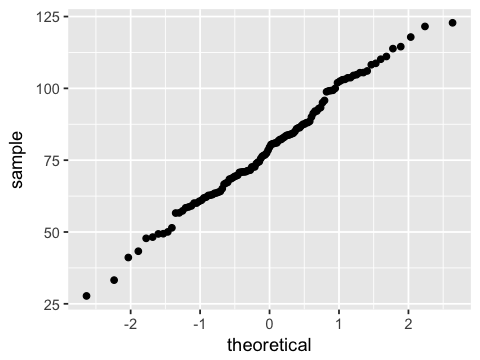
Testing for normality
This is most commonly done visually with a QQ-plot of percentiles of sample versus percentiles of a standard normal distribution. If the sample distribution is normal, you should see a straight diagonal line.
An alternative is the Shapiro-Wilk test for normality.
For testing equal variance, you can use the var.test function in R.
df <- data.frame(x=x)
ggplot(df, aes(sample=x)) + stat_qq()
shapiro.test(df$x)
    Shapiro-Wilk normality test

data:  df$x
W = 0.99162, p-value = 0.6905
var.test(x, y)
    F test to compare two variances

data:  x and y
F = 0.81959, num df = 118, denom df = 116, p-value = 0.283
alternative hypothesis: true ratio of variances is not equal to 1
95 percent confidence interval:
 0.5692599 1.1793311
sample estimates:
ratio of variances
         0.8195921
Exercise
suppressPackageStartupMessages(library(MASS))
data(anorexia)
head(anorexia)
| Treat | Prewt | Postwt |
|---|---|---|
| Cont | 80.7 | 80.2 |
| Cont | 89.4 | 80.1 |
| Cont | 91.8 | 86.4 |
| Cont | 74.0 | 86.3 |
| Cont | 78.1 | 76.1 |
| Cont | 88.3 | 78.1 |
str(anorexia)
'data.frame':       72 obs. of  3 variables:
 $ Treat : Factor w/ 3 levels "CBT","Cont","FT": 2 2 2 2 2 2 2 2 2 2 ...
 $ Prewt : num  80.7 89.4 91.8 74 78.1 88.3 87.3 75.1 80.6 78.4 ...
 $ Postwt: num  80.2 80.1 86.4 86.3 76.1 78.1 75.1 86.7 73.5 84.6 ...
ggplot(anorexia %>% gather(Time, Wt, -Treat), aes(y=Wt, x=Treat, fill=Time)) +
geom_boxplot()
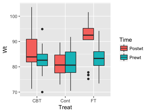
1. There are 3 treatment groups for the anorexia data set. Calculate the confidence intervals and p-values for each treatment using the appropriate T test.
2 Check if the normality assumptions are met for each treatment group.