Statistics review 6: Nonparametric methods
R code accompanying paper
Key learning points
- Common nonparametric methods
- Advantages and disadvantages of nonparametric versus parametric methods
suppressPackageStartupMessages(library(tidyverse))
options(repr.plot.width=4, repr.plot.height=3)
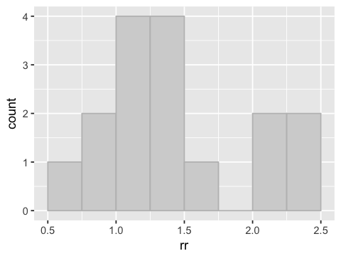
The sign test
rr <- c(0.75, 2.03, 2.29, 2.11, 0.80, 1.50, 0.79, 1.01,
        1.23, 1.48, 2.45, 1.02, 1.03, 1.30, 1.54, 1.27)
ggplot(data.frame(rr=rr), aes(x=rr)) +
geom_histogram(breaks=seq(0.5, 2.5, 0.25), color='gray', fill='lightgray')
n <- length(rr)
k <- sum(rr > 1)
p <- 0.5
S <- min(k, n-k)
S
Calculation of p value from binomial distribution
How likely are we to see 3 heads or fewer in 16 tosses of a fair coin? This is the p-value (double for two-sided test).
round(2 * pbinom(S, n, p), 2)
This is the same as summing the probabilities for 0, 1, 2, and 3 heads.
round(2 * sum(dbinom(0:S, n, p)), 2)
Sign test for paired data
before <- c(39.7, 59.1, 56.1, 57.7, 60.6, 37.8, 58.2, 33.6, 56.0, 65.3)
after <- c(52.9, 56.7, 61.9, 71.4, 67.7, 50.0, 60.7, 51.3, 59.5, 59.8)

df <- data.frame("Subject" = 1:length(before), "Before" = before, "After" = after)
df
| Subject | Before | After |
|---|---|---|
| 1 | 39.7 | 52.9 |
| 2 | 59.1 | 56.7 |
| 3 | 56.1 | 61.9 |
| 4 | 57.7 | 71.4 |
| 5 | 60.6 | 67.7 |
| 6 | 37.8 | 50.0 |
| 7 | 58.2 | 60.7 |
| 8 | 33.6 | 51.3 |
| 9 | 56.0 | 59.5 |
| 10 | 65.3 | 59.8 |
d <- df$After - df$Before
n <- length(d)
k <- sum(d > 0)
S <- min(k, n-k)
round(2 * pbinom(S, n, p), 2)
At the cost of assuming data follow a normal distribution.
t.test(d)
    One Sample t-test

data:  d
t = 2.8681, df = 9, p-value = 0.01853
alternative hypothesis: true mean is not equal to 0
95 percent confidence interval:
  1.432413 12.127587
sample estimates:
mean of x
     6.78
The Wilcoxon signed rank test
df$Difference <- d
df <- df %>% mutate(rank=rank(abs(Difference))) %>%
mutate(sign=sign(Difference)) %>%
arrange(rank)
df
| Subject | Before | After | Difference | rank | sign |
|---|---|---|---|---|---|
| 2 | 59.1 | 56.7 | -2.4 | 1 | -1 |
| 7 | 58.2 | 60.7 | 2.5 | 2 | 1 |
| 9 | 56.0 | 59.5 | 3.5 | 3 | 1 |
| 10 | 65.3 | 59.8 | -5.5 | 4 | -1 |
| 3 | 56.1 | 61.9 | 5.8 | 5 | 1 |
| 5 | 60.6 | 67.7 | 7.1 | 6 | 1 |
| 6 | 37.8 | 50.0 | 12.2 | 7 | 1 |
| 1 | 39.7 | 52.9 | 13.2 | 8 | 1 |
| 4 | 57.7 | 71.4 | 13.7 | 9 | 1 |
| 8 | 33.6 | 51.3 | 17.7 | 10 | 1 |
df %>% filter(sign == 1) %>% summarise(Rp = sum(rank))
| Rp |
|---|
| 50 |
df %>% filter(sign == -1) %>% summarise(Rn = sum(rank))
| Rn |
|---|
| 5 |
There is no simple closed form distribution for the test statistic R, so we’ll just use the built-in R function.
wilcox.test(df$After, df$Before, paired=TRUE)
    Wilcoxon signed rank test

data:  df$After and df$Before
V = 50, p-value = 0.01953
alternative hypothesis: true location shift is not equal to 0
The Wilcoxon rank sum or Mann–Whitney test
dose <- c(7.2, 15.7, 19.1, 21.6, 26.8, 27.4, 28.5, 32.8, 36.3, 43.2, 44.7,
          5.6, 14.6, 18.2, 21.6, 23.1, 28.3, 31.7, 32.4, 36.8)
grp <- c(rep("Nonprotocolized", 11), rep("Protocolized", 9))
df <- data.frame(dose=dose, grp=grp)
df <- df %>% mutate(rank=rank(dose))
df
| dose | grp | rank |
|---|---|---|
| 7.2 | Nonprotocolized | 2.0 |
| 15.7 | Nonprotocolized | 4.0 |
| 19.1 | Nonprotocolized | 6.0 |
| 21.6 | Nonprotocolized | 7.5 |
| 26.8 | Nonprotocolized | 10.0 |
| 27.4 | Nonprotocolized | 11.0 |
| 28.5 | Nonprotocolized | 13.0 |
| 32.8 | Nonprotocolized | 16.0 |
| 36.3 | Nonprotocolized | 17.0 |
| 43.2 | Nonprotocolized | 19.0 |
| 44.7 | Nonprotocolized | 20.0 |
| 5.6 | Protocolized | 1.0 |
| 14.6 | Protocolized | 3.0 |
| 18.2 | Protocolized | 5.0 |
| 21.6 | Protocolized | 7.5 |
| 23.1 | Protocolized | 9.0 |
| 28.3 | Protocolized | 12.0 |
| 31.7 | Protocolized | 14.0 |
| 32.4 | Protocolized | 15.0 |
| 36.8 | Protocolized | 18.0 |
df %>% filter(grp == "Protocolized") %>% summarise(sum=sum(rank))
| sum |
|---|
| 84.5 |
x <- df %>% filter(grp == "Protocolized") %>% select(dose)
y <- df %>% filter(grp == "Nonprotocolized") %>% select(dose)
wilcox.test(x[,], y[,])
Warning message in wilcox.test.default(x[, ], y[, ]):
“cannot compute exact p-value with ties”
    Wilcoxon rank sum test with continuity correction

data:  x[, ] and y[, ]
W = 39.5, p-value = 0.4703
alternative hypothesis: true location shift is not equal to 0
t.test(x, y)
    Welch Two Sample t-test

data:  x and y
t = -0.83661, df = 17.926, p-value = 0.4138
alternative hypothesis: true difference in means is not equal to 0
95 percent confidence interval:
 -13.991115   6.023438
sample estimates:
mean of x mean of y
 23.58889  27.57273
Advantages of nonparametric methods
- Nonparametric methods require no or very limited assump- tions to be made about the format of the data, and they may therefore be preferable when the assumptions required for parametric methods are not valid.
- Nonparametric methods can be useful for dealing with unex- pected, outlying observations that might be problematic with a parametric approach.
- Nonparametric methods are intuitive and are simple to carry out by hand, for small samples at least.
- Nonparametric methods are often useful in the analysis of ordered categorical data in which assignation of scores to individual categories may be inappropriate.
Disadvantages of nonparametric methods
- Nonparametric methods may lack power as compared with more traditional approaches.
- Nonparametric methods are geared toward hypothesis testing rather than estimation of effects.
- Tied values can be problematic when these are common.