Statistics review 8: Qualitative data – tests of association
R code accompanying paper)
Key learning points
- How to investigate relationships between two qualitative (categorical) variables
- \(\chi^2\) test of association
- Test for trend (one variable is ordinal)
- Risk measurement
- Evaluating proportions
suppressPackageStartupMessages(library(tidyverse))
options(repr.plot.width=4, repr.plot.height=3)
Categorical data
Unordered
- sex
- blood group
- classification of disease
- whether the patient survived
Ordinal
- Age group
- Clinical scales (e.g. Pain scale)
\(\chi^2\) test of association
none <-  c(686, 451, 168)
exit <- c(152, 35, 58)
bacteremia <- c(96, 38, 22)

o <- data.frame(none=none, exit=exit, bacteremia=bacteremia,
                row.names= c("jugular", "subclavian", "femoral"))
Observed counts
o
| none | exit | bacteremia | |
|---|---|---|---|
| jugular | 686 | 152 | 96 |
| subclavian | 451 | 35 | 38 |
| femoral | 168 | 58 | 22 |
m <- addmargins(as.matrix(o))
m
| none | exit | bacteremia | Sum | |
|---|---|---|---|---|
| jugular | 686 | 152 | 96 | 934 |
| subclavian | 451 | 35 | 38 | 524 |
| femoral | 168 | 58 | 22 | 248 |
| Sum | 1305 | 245 | 156 | 1706 |
Expected counts
e <- outer(m[1:3,4], m[4,1:3]/m[4,4])
round(e, 1)
| none | exit | bacteremia | |
|---|---|---|---|
| jugular | 714.5 | 134.1 | 85.4 |
| subclavian | 400.8 | 75.3 | 47.9 |
| femoral | 189.7 | 35.6 | 22.7 |
Calculate \(\chi^2\) test statistic
T <- sum((o - e)^2/e)
round(T, 2)
df <- (nrow(o) -1) * (ncol(o)  - 1)
df
Calculate p-value from \(\chi^2\) distribution
1 - pchisq(T, df)
Use built in test
chisq.test(o)
    Pearson's Chi-squared test

data:  o
X-squared = 51.262, df = 4, p-value = 1.968e-10
Residuals
t <- addmargins(as.matrix(prop.table(o)))
t
| none | exit | bacteremia | Sum | |
|---|---|---|---|---|
| jugular | 0.40211020 | 0.08909730 | 0.05627198 | 0.5474795 |
| subclavian | 0.26436108 | 0.02051583 | 0.02227433 | 0.3071512 |
| femoral | 0.09847597 | 0.03399766 | 0.01289566 | 0.1453693 |
| Sum | 0.76494725 | 0.14361079 | 0.09144197 | 1.0000000 |
Adjusted standardized residues
The numbers don’t agree with table 4 in the paper. Student to check by hand calculations?
round((o - e)/sqrt(e*(1-t[1:3,4])*(1-t[4,1:3])), 1)
| none | exit | bacteremia | |
|---|---|---|---|
| jugular | -3.3 | 4.7 | 3.5 |
| subclavian | 3.3 | -6.0 | -1.9 |
| femoral | -1.8 | 4.3 | -0.2 |
Two by two tables
treatment <- c(3, 47)
control <- c(8, 37)
df1 <- data.frame(treatment=treatment, contorl=control)
df1
| treatment | contorl |
|---|---|
| 3 | 8 |
| 47 | 37 |
chisq.test(df1, correct = FALSE)
    Pearson's Chi-squared test

data:  df1
X-squared = 3.2089, df = 1, p-value = 0.07324
Fisher’s exact test
fisher.test(df1)
    Fisher's Exact Test for Count Data

data:  df1
p-value = 0.1083
alternative hypothesis: true odds ratio is not equal to 1
95 percent confidence interval:
 0.04775944 1.35642029
sample estimates:
odds ratio
 0.2989279
Yates’ continuity correction
chisq.test(df1, correct=TRUE)
    Pearson's Chi-squared test with Yates' continuity correction

data:  df1
X-squared = 2.1617, df = 1, p-value = 0.1415
Test for trend
alert <- c(1110, 108)
vopr <- c(54, 14)
unresponsive <- c(14, 6)
df2 <- data.frame(alert=alert, vopr=vopr, unresponsive=unresponsive,
                  row.names=c("sruvived", "died"))
df2
| alert | vopr | unresponsive | |
|---|---|---|---|
| sruvived | 1110 | 54 | 14 |
| died | 108 | 14 | 6 |
chisq.test(df2)
Warning message in chisq.test(df2):
“Chi-squared approximation may be incorrect”
    Pearson's Chi-squared test

data:  df2
X-squared = 19.383, df = 2, p-value = 6.18e-05
Calling the trend test
The trend test takes two arguments
- Number of events
- Number of trials
So we have to a little massaging to get the data in the correct format.
We can use either row as the number of events
Using number of survivors.
prop.trend.test(as.matrix(df2[1,]), colSums(df2))
    Chi-squared Test for Trend in Proportions

data:  as.matrix(df2[1, ]) out of colSums(df2) ,
 using scores: 1 2 3
X-squared = 19.328, df = 1, p-value = 1.101e-05
Using number of deaths.
prop.trend.test(as.matrix(df2[2,]), colSums(df2))
    Chi-squared Test for Trend in Proportions

data:  as.matrix(df2[2, ]) out of colSums(df2) ,
 using scores: 1 2 3
X-squared = 19.328, df = 1, p-value = 1.101e-05
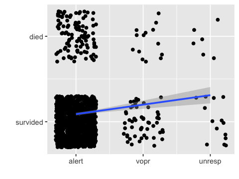
Interpretation as slope of linear regression model
points <- c(replicate(1110, c(1,1)), replicate(108, c(1,2)),
            replicate(54, c(2,1)),  replicate(14, c(2,2)),
            replicate(14, c(3,1)), replicate(6, c(3,2)))
length(points)
df3 <- data.frame(matrix(points, ncol=2, byrow = T))
colnames(df3) <- c("x", "y")
summary(lm(y ~ x - 1 , data=df3))
Call:
lm(formula = y ~ x - 1, data = df3)

Residuals:
     Min       1Q   Median       3Q      Max
-1.81677  0.06108  0.06108  0.06108  1.06108

Coefficients:
  Estimate Std. Error t value Pr(>|t|)
x 0.938922   0.009996   93.93   <2e-16 *
---
Signif. codes:  0 ‘*’ 0.001 ‘**’ 0.01 ‘*’ 0.05 ‘.’ 0.1 ‘ ’ 1

Residual standard error: 0.4085 on 1305 degrees of freedom
Multiple R-squared:  0.8711,        Adjusted R-squared:  0.871
F-statistic:  8822 on 1 and 1305 DF,  p-value: < 2.2e-16
ggplot(df3, aes(x=x, y=y)) + geom_jitter(width = .3, height=.3) +
geom_smooth(method="lm") +
scale_x_continuous(breaks=1:3, labels=c("alert", "vopr", "unresp")) +
scale_y_continuous(breaks=1:2, labels=c("survided", "died")) +
xlab("") + ylab("")
Measurement of risk
died <- c(38, 59)
survived <- c(79, 60)
df4 <- data.frame(died=died, survived=survived, row.names=c("early", "standard"))
df4
| died | survived | |
|---|---|---|
| early | 38 | 79 |
| standard | 59 | 60 |
round(100*df4[1,1]/sum(df4[1,]), 1)
round(100*df4[2,1]/sum(df4[2,]), 1)
round(df4[1,1]/sum(df4[1,2]), 2)
round(df4[2,1]/sum(df4[2,2]), 2)
Confidence interval for a proportion
Confidence interval for death with early treatment
n <- sum(df4[1,])
p <- df4[1,1]/n
alpha <- 0.05
k <- qnorm(1 - alpha/2)
se <- sqrt(p*(1-p)/n)
round(100*c(p - k*se, p + k*se), 1)
- 24
- 41
Confidence interval for death with early treatment
n <- sum(df4[2,])
p <- df4[2,1]/n
alpha <- 0.05
k <- qnorm(1 - alpha/2)
se <- sqrt(p*(1-p)/n)
round(100*c(p - k*se, p + k*se), 1)
- 40.6
- 58.6
Testing for difference between two proportions
df4
| died | survived | |
|---|---|---|
| early | 38 | 79 |
| standard | 59 | 60 |
df4 <- df4 %>% mutate(total=died+survived)
df4
| died | survived | total |
|---|---|---|
| 38 | 79 | 117 |
| 59 | 60 | 119 |
prop.test(df4[,1], df4[,3], correct = FALSE)
    2-sample test for equality of proportions without continuity
    correction

data:  df4[, 1] out of df4[, 3]
X-squared = 7.1271, df = 1, p-value = 0.007593
alternative hypothesis: two.sided
95 percent confidence interval:
 -0.29458384 -0.04744015
sample estimates:
   prop 1    prop 2
0.3247863 0.4957983
Matched samples
breath_plus <- c(40, 4)
breath_minus <- c(8, 32)
df5 <- data.frame(breath_plus=breath_plus, breath_minus=breath_minus,
                 row.names=c("xxoid_plus", "oxoid_minus"))
df5
| breath_plus | breath_minus | |
|---|---|---|
| xxoid_plus | 40 | 8 |
| oxoid_minus | 4 | 32 |
Using built in test
mcnemar.test(as.matrix(df5))
    McNemar's Chi-squared test with continuity correction

data:  as.matrix(df5)
McNemar's chi-squared = 0.75, df = 1, p-value = 0.3865
Exercises
suppressPackageStartupMessages(library(MASS))
The rows indicate smoking history, and the columns indicate frequency of exercise
The allowed values in Smoke are “Heavy”, “Regul” (regularly), “Occas” (occasionally) and “Never”, and “Freq” (frequently), “Some” and “None” for Exercise.
tbl = table(survey$Smoke, survey$Exer)
tbl
      Freq None Some
Heavy    7    1    3
Never   87   18   84
Occas   12    3    4
Regul    9    1    7
1. Is there a evidence for a relationship between smoking history and frequency of exercise? Solve this a) by manual calculation, and b) by using the chisq.test.
2. Is there evidence for a trend for exercise with frequency of smoking if we consider smoking as an ordinal variables?
3. Create a new table that uses only the (Freq, None) columns and (Heavy, Never) rows. Compare the results of the \(\chi^2\) test with and without Yates continuity correction, as well as the Fisher exact test.