Statistics review 7: Correlation and regression

R code accompanying paper

Key learning points

• Correlation quantifies the strength of the linear relationship between a pair of variables
• Regression expresses the relationship in the form of an equation

suppressPackageStartupMessages(library(tidyverse))

options(repr.plot.width=4, repr.plot.height=3)

Scatter diagram

age <- c(60, 76, 81, 89, 44, 58, 55, 74, 45, 67, 72,
         91, 76, 39, 71, 56, 77, 37, 64, 84)
urea <- c(1.099, 1.723, 2.054, 2.262, 1.686, 1.988, 1.131, 1.917, 1.548, 1.386,
              2.617, 2.701, 2.054, 1.526, 2.002, 1.526, 1.825, 1.435, 2.460, 1.932)

ae <- data.frame(subject=1:20, age=age, urea=urea)

head(ae)

subject	age	urea
1	60	1.099
2	76	1.723
3	81	2.054
4	89	2.262
5	44	1.686
6	58	1.988

ggplot(ae, aes(x=age, y=urea)) + geom_point()

Correlation

Function to calculate Pearson’s correlatin

pearson <- function(x, y) {
    xbar <- mean(x)
    ybar <- mean(y)
    sum((x - xbar)*(y-ybar))/sqrt(sum((x-xbar)^2)*sum((y-ybar)^2))
}

round(pearson(x=ae$age, y=ae$urea), 2)

0.62

Using built-in function

round(cor(x=ae$age, y=ae$urea, method = 'pearson'), 2)

0.62

Hypothesis test of correlation

cor.test(x=ae$age, y=ae$urea)

    Pearson's product-moment correlation

data:  ae$age and ae$urea
t = 3.3538, df = 18, p-value = 0.003535
alternative hypothesis: true correlation is not equal to 0
95 percent confidence interval:
 0.2447935 0.8338342
sample estimates:
      cor
0.6201371

Confidence interval for the population correlation coefficient

This is also provided by the built in test function.

z <- c(0.5 * log((1+0.62)/(1 - 0.62)))
se <- 1/sqrt(20 -3)

z.ci <- c(z - 1.96*se, z + 1.96*se)
round(z.ci, 2)

1. 0.25
2. 1.2

ci <- c((exp(2*z.ci[1]) - 1)/(exp(2*z.ci[1]) + 1),
        (exp(2*z.ci[2]) - 1)/(exp(2*z.ci[2]) + 1))
round(ci, 2)

1. 0.24
2. 0.83

Misuse of correlation

Correlations may arise from third variable

z <- 3*rnorm(10)
x <- z + rnorm(10)
y <- z + rnorm(10)

df <- data.frame(x=x, y=y)

ggplot(df, aes(x=x, y=y)) + geom_point() + geom_smooth(method=lm) +
annotate("text", x=-4, y=5, label = paste("r =", round(cor(df$x, df$y), 2)))

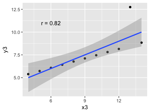
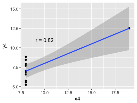
Correlations can be misleading if relationships are non-linear

head(anscombe)

x1	x2	x3	x4	y1	y2	y3	y4
10	10	10	8	8.04	9.14	7.46	6.58
8	8	8	8	6.95	8.14	6.77	5.76
13	13	13	8	7.58	8.74	12.74	7.71
9	9	9	8	8.81	8.77	7.11	8.84
11	11	11	8	8.33	9.26	7.81	8.47
14	14	14	8	9.96	8.10	8.84	7.04

g1 <- ggplot(anscombe, aes(x=x1, y=y1)) +
geom_point() + geom_smooth(method=lm) +
annotate("text", x=6, y=9,
         label = paste("r =", round(cor(anscombe$x1, anscombe$y1), 2)))
g2 <- ggplot(anscombe, aes(x=x2, y=y2)) +
geom_point() + geom_smooth(method=lm) +
annotate("text", x=6, y=9,
         label = paste("r =", round(cor(anscombe$x2, anscombe$y2), 2)))
g3 <- ggplot(anscombe, aes(x=x3, y=y3)) +
geom_point() + geom_smooth(method=lm) +
annotate("text", x=6, y=11,
         label = paste("r =", round(cor(anscombe$x3, anscombe$y3), 2)))
g4 <- ggplot(anscombe, aes(x=x4, y=y4)) +
geom_point() + geom_smooth(method=lm) +
annotate("text", x=10, y=11,
         label = paste("r =", round(cor(anscombe$x4, anscombe$y4), 2)))

g1

g2

g3

g4

Correlations may arise from subgroups

m <- rnorm(10, 70, 4)
f <- rnorm(10, 65, 3.5)
x.m <- rnorm(10, 0)
x.f <- rnorm(10, 6)

df <- data.frame(x=c(x.f, x.m), height=c(f, m),
                 sex=c(rep("f", 10), rep("m", 10)))

ggplot(df, aes(x=x, y=height)) + geom_point() +
geom_smooth(method=lm) +
annotate("text", x=6, y=72,
         label = paste("r =", round(cor(df$x, df$height), 2)))

Regression

x <- ae$age
xbar <- mean(x)
y <- ae$urea
ybar <- mean(y)

b <- sum((x - xbar)*(y - ybar))/sum((x-xbar)^2)
a <- ybar - b*xbar
round(c(a, b), 4)

1. 0.7147
2. 0.0172

ggplot(ae, aes(x=age, y=urea)) + geom_point() +
geom_abline(aes(intercept=a, slope=b), color="blue")

Hypothesis tests and confidence intervals

fit <- lm(urea ~ age, data=ae)
summary(fit)

Call:
lm(formula = urea ~ age, data = ae)

Residuals:
     Min       1Q   Median       3Q      Max
-0.64509 -0.21403  0.02789  0.16075  0.66703

Coefficients:
            Estimate Std. Error t value Pr(>|t|)
(Intercept) 0.714698   0.346129   2.065  0.05365 .
age         0.017157   0.005116   3.354  0.00354 **
---
Signif. codes:  0 ‘*’ 0.001 ‘’ 0.01 ‘*’ 0.05 ‘.’ 0.1 ‘ ’ 1

Residual standard error: 0.3606 on 18 degrees of freedom
Multiple R-squared:  0.3846,        Adjusted R-squared:  0.3504
F-statistic: 11.25 on 1 and 18 DF,  p-value: 0.003535

cor.test(ae$age, ae$urea)

    Pearson's product-moment correlation

data:  ae$age and ae$urea
t = 3.3538, df = 18, p-value = 0.003535
alternative hypothesis: true correlation is not equal to 0
95 percent confidence interval:
 0.2447935 0.8338342
sample estimates:
      cor
0.6201371

Analysis of variance

anova

fit.aov <- anova(fit)
fit.aov

	Df	Sum Sq	Mean Sq	F value	Pr(>F)
age	1	1.462673	1.4626726	11.24785	0.003535245
Residuals	18	2.340724	0.1300402	NA	NA

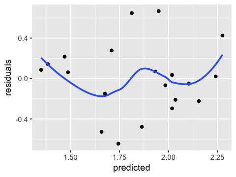
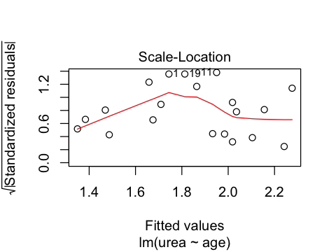
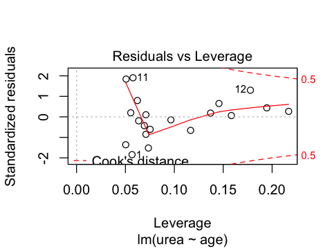
Residuals

ae$predicted <- predict(fit)
ae$residuals <- residuals(fit)

ggplot(ae, aes(x = age, y = urea)) +
  geom_smooth(method = "lm", se = FALSE, color = "lightgrey") +  # Plot regression slope
  geom_segment(aes(xend = age, yend = predicted), alpha = .2) +  # alpha to fade lines
  geom_point() +
  geom_point(aes(y = predicted), shape = 1)

Coefficient of determination

Regression_sum_of_squares <- fit.aov$'Sum Sq'[1]
Total_sum_of_squares <- fit.aov$'Sum Sq'[2]
round(c(Regression_sum_of_squares, Total_sum_of_squares), 4)

1. 1.4627
2. 2.3407

Explained variance

Age accounts for 38% of the total varia- tion in ln urea

r_squared = (Regression_sum_of_squares/Total_sum_of_squares)^2
round(r_squared, 2)

0.39

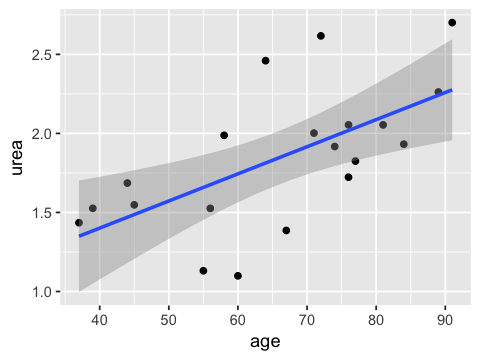
Prediction

newdata <- data.frame(age = seq(40, 90, 10))
newdata$urea.pred <- predict(fit, newdata)
newdata

age	urea.pred
40	1.400961
50	1.572526
60	1.744092
70	1.915658
80	2.087223
90	2.258789

ggplot(ae, aes(x=age, y=urea)) + geom_point() + geom_smooth(method=lm, )

names(fit)

1. 'coefficients'
2. 'residuals'
3. 'effects'
4. 'rank'
5. 'fitted.values'
6. 'assign'
7. 'qr'
8. 'df.residual'
9. 'xlevels'
10. 'call'
11. 'terms'
12. 'model'

ggplot(ae, aes(x=predicted, y=residuals)) +
geom_point() + geom_smooth(se=FALSE)

geom_smooth() using method = 'loess'

ggplot(ae, aes(sample=residuals)) + stat_qq()

Default diagnostic plots

plot(fit)

Exercises

You may need to install the car package in R in the usual way:

install.packages("car")

suppressPackageStartupMessages(library(car))

head(Davis)

sex	weight	height	repwt	repht
M	77	182	77	180
F	58	161	51	159
F	53	161	54	158
M	68	177	70	175
F	59	157	59	155
M	76	170	76	165

1. Find the correlation between age and height for males and females in the Davis data set.

2. Test if the correlation is significant.

3. Repeat exercises 1 and 2 taking for each sex spearately.

4. Show separate linear regressions of weight (y-axis) on height (x-axis) for each sex, either on the same plot (using different colors) or on different subplots.

5. What is the predicted weight of a female who is 165 cm tall?