Statistics review 13: Receiver operating characteristic

R code accompanying paper

Key learning points

• Methods for assessing the performance of a diagnostic test
• Sensitivity, specificity and likelihood ratio of a test
• Receiver operating characteristic curve and the area under the curve

suppressPackageStartupMessages(library(tidyverse))

options(repr.plot.width=4, repr.plot.height=3)

Data

died <- c(81, 45)
survived <- c(591, 674)

df1 <- data.frame(died=died, survived=survived,
                  row.names=c("Lactate >1.5 mmol/l", "Lactate ≤1.5 mmol/l"))
df1

	died	survived
Lactate >1.5 mmol/l	81	591
Lactate ≤1.5 mmol/l	45	674

Data set with different prevalence

died <- c(386, 214)
survived <- c(370, 421)

df2 <- data.frame(died=died, survived=survived,
                  row.names=c("Lactate >1.5 mmol/l", "Lactate ≤1.5 mmol/l"))
df2

	died	survived
Lactate >1.5 mmol/l	386	370
Lactate ≤1.5 mmol/l	214	421

Sensitivity and specificity

prop.ci <- function(p, n, alpha=0.05) {
    se <- sqrt(p*(1-p)/n)
    k <- qnorm(1 - alpha/2)
    round(c(p - k*se, p + k*se), 2)
}

sens <- function(tbl) {
    a <- tbl[1,1]
    b <- tbl[1,2]
    c <- tbl[2,1]
    d <- tbl[2,2]
    n <- a + c
    p <- a/n

    round(p, 2)
}

sens(df1)

0.64

p <- sens(df1)
n <- sum(df1)
prop.ci(p, n)

1. 0.61
2. 0.67

spec <- function(tbl) {
    a <- tbl[1,1]
    b <- tbl[1,2]
    c <- tbl[2,1]
    d <- tbl[2,2]
    n <- b + d

    p <- d/n
    round(p, 2)
}

spec(df1)

0.53

Positive and negative predictive values

ppv <- function(tbl) {
    a <- tbl[1,1]
    b <- tbl[1,2]
    c <- tbl[2,1]
    d <- tbl[2,2]
    n <- a + b
    p <- a/n

    round(p, 2)
}

ppv(df1)

0.12

npv <- function(tbl, alpha=0.05) {
    a <- tbl[1,1]
    b <- tbl[1,2]
    c <- tbl[2,1]
    d <- tbl[2,2]
    n <- c + d

    p <- d/n
    round(p, 2)
}

npv(df1)

0.94

Effect of prevalence

c(sens(df1)[1], sens(df2)[1])

1. 0.64
2. 0.64

c(spec(df1)[1], spec(df2)[1])

1. 0.53
2. 0.53

c(ppv(df1)[1], ppv(df2)[1])

1. 0.12
2. 0.51

c(npv(df1)[1], npv(df2)[1])

1. 0.94
2. 0.66

Likelihood ratios

lr <- function(tbl) {
    round(sens(tbl)[1]/(1 - spec(tbl)[1]), 2)
}

lr(df1)

1.36

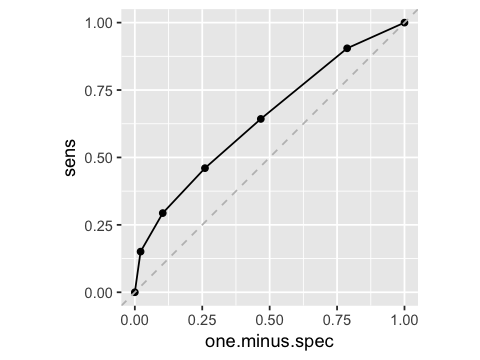
Receiver operating characteristic curve (ROC)

threshold <- c(0,1,1.5,2,3,5,25)
died <- c(126,114,81,58,37,19,0)
survived <- c(1265,996,591,329,131,27,0)

df3 <- data.frame(threshold=threshold, died=died, survived=survived)
df3

threshold	died	survived
0.0	126	1265
1.0	114	996
1.5	81	591
2.0	58	329
3.0	37	131
5.0	19	27
25.0	0	0

n.died <- 126
n.survived <- 1265

sens.1 <-function(died, ndied) {
    a <- died
    c <- ndied-died
    a/(a + c)
}

spec.1 <-function(survived, nsurvived) {
    b <- survived
    d <- nsurvived - survived
    b/(b+d)
}

df4 <- df3 %>% mutate(sens=sens.1(died, n.died), one.minus.spec=spec.1(survived, n.survived))
df4

threshold	died	survived	sens	one.minus.spec
0.0	126	1265	1.0000000	1.00000000
1.0	114	996	0.9047619	0.78735178
1.5	81	591	0.6428571	0.46719368
2.0	58	329	0.4603175	0.26007905
3.0	37	131	0.2936508	0.10355731
5.0	19	27	0.1507937	0.02134387
25.0	0	0	0.0000000	0.00000000

ggplot(df4, aes(x=one.minus.spec, y=sens)) + geom_point() + geom_line() +
geom_abline(intercept = 0, slope = 1, color='grey', linetype='dashed') +
coord_fixed()

Area under the curve (AUCROC)

suppressPackageStartupMessages(require(pracma))

round(-1 * trapz(x=df4$one.minus.spec, y=df4$sens), 2)

0.64