Statistics review 14: Logistic regression

R code accompanying paper

Key learning points

• Modeling the dependence of a binary response variable on one or more explanatory variables

suppressPackageStartupMessages(library(tidyverse))

options(repr.plot.width=4, repr.plot.height=3)

marker <- seq(0.75, 4.75, by=0.5)
patients <- c(182, 233, 224, 236, 225, 215, 221, 200, 264)
deaths <- c(7, 27, 44, 91, 130, 168, 194, 191, 260)

df <- data.frame(marker=marker, patients=patients, deaths=deaths)
df

marker	patients	deaths
0.75	182	7
1.25	233	27
1.75	224	44
2.25	236	91
2.75	225	130
3.25	215	168
3.75	221	194
4.25	200	191
4.75	264	260

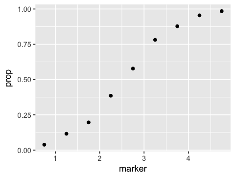
df1 <- df %>% mutate(prop=deaths/patients)
df1

marker	patients	deaths	prop
0.75	182	7	0.03846154
1.25	233	27	0.11587983
1.75	224	44	0.19642857
2.25	236	91	0.38559322
2.75	225	130	0.57777778
3.25	215	168	0.78139535
3.75	221	194	0.87782805
4.25	200	191	0.95500000
4.75	264	260	0.98484848

ggplot(df1, aes(x=marker, y=prop)) + geom_point()

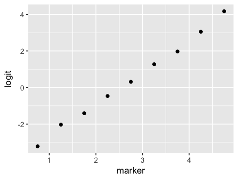
df2 <- df1 %>% mutate(logit=log(prop/(1-prop)))
df2

marker	patients	deaths	prop	logit
0.75	182	7	0.03846154	-3.2188758
1.25	233	27	0.11587983	-2.0320393
1.75	224	44	0.19642857	-1.4087672
2.25	236	91	0.38559322	-0.4658742
2.75	225	130	0.57777778	0.3136576
3.25	215	168	0.78139535	1.2738164
3.75	221	194	0.87782805	1.9720213
4.25	200	191	0.95500000	3.0550489
4.75	264	260	0.98484848	4.1743873

ggplot(df2, aes(x=marker, y=logit)) + geom_point()

Maximum likelihood estimation

The parameters of many statistical models are estimated by maximizing the likelihood. This likelihood is a function of the unnormalized probability density after having observed some data. We will illustrate by example to give some intuition.

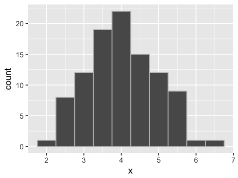
Simulating sample data come from a population

mu <- 4
sigma <- 1
x <- rnorm(100, mu, sigma)

ggplot(data.frame(x=x), aes(x=x)) + geom_histogram(binwidth=0.5, color='grey')

Likelihood

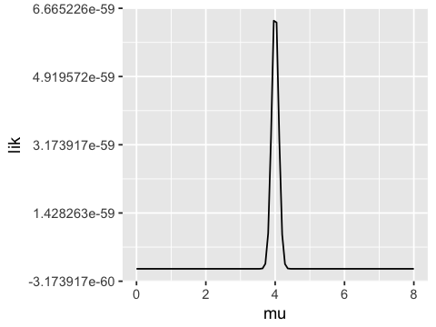
We have 100 samples independently drawn from the same normal distribution - that is, the samples are IID (independent identically distributed). The conditional probability of of a single sample \(x_i\) is \(N(\mu, \sigma \mid x_i)\). Because the samples are independent, the likelihood of seeing all 100 samples is just the product of 100 such conditional probabilities.

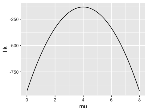
If we fix the standard deviation to be 1 and vary the mean, we see that the likelihood function has a maximum near the true population mean (\(\mu = 4\)). Hence we can get a good estimate of \(\mu\) by maximizing the likelihood. Typically, a numerical optimization algorithm is used to find the maximum - the value of \(\mu\) (or other parameter) where this maximum occurs is the maximum likelihood estimate (MLE) of the population parameter.

mus <- seq(0, 8, length.out = 100)
lik <- vector('numeric', length=100)
for (i in 1:100) {
    lik[i] <- prod(dnorm(x, mean=mus[i], sd=1))
}

ggplot(data.frame(mu=mus, lik=lik), aes(x=mu, y=lik)) + geom_line()

Working in log space

In practice, multiplying lots of small numbers to get a likelihood results in underflow because of the discreteness of computer arithmetic. So we work with log probabilities and sum them rather than take products, but the basic idea of maximizing the (log) likelihood is the same.

mus <- seq(0, 8, length.out = 100)
loglik <- vector('numeric', length=100)
for (i in 1:100) {
    loglik[i] <- sum(log(dnorm(x, mean=mus[i], sd=1)))
}

ggplot(data.frame(mu=mus, lik=loglik), aes(x=mu, y=lik)) + geom_line()

Data with binary outcomes

We will try to predict admission to graduate school based on GRE, GPA and class rank. Rank is the prestige of the undergraduate institution, with 1 = most prestigious and 4 = least prestigious.

admit <- read.csv("http://stats.idre.ucla.edu/stat/data/binary.csv")

admit$rank <- as.factor(admit$rank)

str(admit)

'data.frame':       400 obs. of  4 variables:
 $ admit: int  0 1 1 1 0 1 1 0 1 0 ...
 $ gre  : int  380 660 800 640 520 760 560 400 540 700 ...
 $ gpa  : num  3.61 3.67 4 3.19 2.93 3 2.98 3.08 3.39 3.92 ...
 $ rank : Factor w/ 4 levels "1","2","3","4": 3 3 1 4 4 2 1 2 3 2 ...

head(admit)

admit	gre	gpa	rank
0	380	3.61	3
1	660	3.67	3
1	800	4.00	1
1	640	3.19	4
0	520	2.93	4
1	760	3.00	2

m <- glm(admit ~ gre + gpa + rank, data=admit, family="binomial")

summary(m)

Call:
glm(formula = admit ~ gre + gpa + rank, family = "binomial",
    data = admit)

Deviance Residuals:
    Min       1Q   Median       3Q      Max
-1.6268  -0.8662  -0.6388   1.1490   2.0790

Coefficients:
             Estimate Std. Error z value Pr(>|z|)
(Intercept) -3.989979   1.139951  -3.500 0.000465 *
gre          0.002264   0.001094   2.070 0.038465 *
gpa          0.804038   0.331819   2.423 0.015388 *
rank2       -0.675443   0.316490  -2.134 0.032829 *
rank3       -1.340204   0.345306  -3.881 0.000104 *
rank4       -1.551464   0.417832  -3.713 0.000205 *
---
Signif. codes:  0 ‘*’ 0.001 ‘**’ 0.01 ‘*’ 0.05 ‘.’ 0.1 ‘ ’ 1

(Dispersion parameter for binomial family taken to be 1)

    Null deviance: 499.98  on 399  degrees of freedom
Residual deviance: 458.52  on 394  degrees of freedom
AIC: 470.52

Number of Fisher Scoring iterations: 4

round(confint(m), 4)

Waiting for profiling to be done...

	2.5 %	97.5 %
(Intercept)	-6.2716	-1.7925
gre	0.0001	0.0044
gpa	0.1603	1.4641
rank2	-1.3009	-0.0567
rank3	-2.0277	-0.6704
rank4	-2.4000	-0.7535

library(aod)

Test significance of GRE

wald.test(b = coef(m), Sigma = vcov(m), Terms = 2)

Wald test:
----------

Chi-squared test:
X2 = 4.3, df = 1, P(> X2) = 0.038

Test significance of GPA

wald.test(b = coef(m), Sigma = vcov(m), Terms = 3)

Wald test:
----------

Chi-squared test:
X2 = 5.9, df = 1, P(> X2) = 0.015

Test significance of Rank

wald.test(b = coef(m), Sigma = vcov(m), Terms = 4:6)

Wald test:
----------

Chi-squared test:
X2 = 20.9, df = 3, P(> X2) = 0.00011

Getting odds ratios

round(exp(cbind(OR = coef(m), confint(m))), 4)

Waiting for profiling to be done...

	OR	2.5 %	97.5 %
(Intercept)	0.0185	0.0019	0.1665
gre	1.0023	1.0001	1.0044
gpa	2.2345	1.1739	4.3238
rank2	0.5089	0.2723	0.9448
rank3	0.2618	0.1316	0.5115
rank4	0.2119	0.0907	0.4707

For every unit increase in GPA, the odds of being admitted increase by a factor of 2.2345.

Making predictions

head(admit)

admit	gre	gpa	rank
0	380	3.61	3
1	660	3.67	3
1	800	4.00	1
1	640	3.19	4
0	520	2.93	4
1	760	3.00	2

new.data <- with(admit, data.frame(gre=mean(gre), gpa=mean(gpa), rank=factor(1:4)))

new.data

gre	gpa	rank
587.7	3.3899	1
587.7	3.3899	2
587.7	3.3899	3
587.7	3.3899	4

new.data$p <- predict(m, new.data, type="response")
new.data

gre	gpa	rank	p
587.7	3.3899	1	0.5166016
587.7	3.3899	2	0.3522846
587.7	3.3899	3	0.2186120
587.7	3.3899	4	0.1846684

Exercise

library(titanic)

head(titanic_train)

PassengerId	Survived	Pclass	Name	Sex	Age	SibSp	Parch	Ticket	Fare	Cabin	Embarked
1	0	3	Braund, Mr. Owen Harris	male	22	1	0	A/5 21171	7.2500		S
2	1	1	Cumings, Mrs. John Bradley (Florence Briggs Thayer)	female	38	1	0	PC 17599	71.2833	C85	C
3	1	3	Heikkinen, Miss. Laina	female	26	0	0	STON/O2. 3101282	7.9250		S
4	1	1	Futrelle, Mrs. Jacques Heath (Lily May Peel)	female	35	1	0	113803	53.1000	C123	S
5	0	3	Allen, Mr. William Henry	male	35	0	0	373450	8.0500		S
6	0	3	Moran, Mr. James	male	NA	0	0	330877	8.4583		Q

str(titanic_train)

'data.frame':       891 obs. of  12 variables:
 $ PassengerId: int  1 2 3 4 5 6 7 8 9 10 ...
 $ Survived   : int  0 1 1 1 0 0 0 0 1 1 ...
 $ Pclass     : int  3 1 3 1 3 3 1 3 3 2 ...
 $ Name       : chr  "Braund, Mr. Owen Harris" "Cumings, Mrs. John Bradley (Florence Briggs Thayer)" "Heikkinen, Miss. Laina" "Futrelle, Mrs. Jacques Heath (Lily May Peel)" ...
 $ Sex        : chr  "male" "female" "female" "female" ...
 $ Age        : num  22 38 26 35 35 NA 54 2 27 14 ...
 $ SibSp      : int  1 1 0 1 0 0 0 3 0 1 ...
 $ Parch      : int  0 0 0 0 0 0 0 1 2 0 ...
 $ Ticket     : chr  "A/5 21171" "PC 17599" "STON/O2. 3101282" "113803" ...
 $ Fare       : num  7.25 71.28 7.92 53.1 8.05 ...
 $ Cabin      : chr  "" "C85" "" "C123" ...
 $ Embarked   : chr  "S" "C" "S" "S" ...

1. Fit a logistic regression model of survival against sex, age, and passenger class (Pclass). Remember to convert to factors as appropriate. Evaluate and interpret the impact of sex, age and passenger class on survival.