Using optimization routines from scipy and statsmodels
In [1]:
import scipy.linalg as la
Finding roots
For root finding, we generally need to proivde a starting point in the vicinitiy of the root. For iD root finding, this is often provided as a bracket (a, b) where a and b have opposite signs.
Univariate roots and fixed points
In [2]:
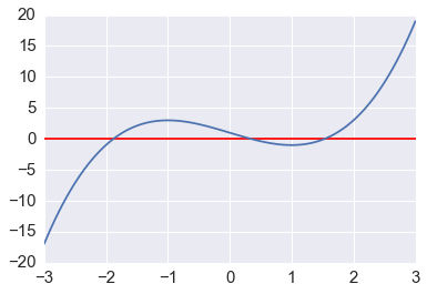
def f(x):
    return x**3-3*x+1
In [3]:
x = np.linspace(-3,3,100)
plt.axhline(0, c='red')
plt.plot(x, f(x));
In [4]:
from scipy.optimize import brentq, newton
brentq is the recommended method
In [5]:
brentq(f, -3, 0), brentq(f, 0, 1), brentq(f, 1,3)
Out[5]:
(-1.8793852415718166, 0.3472963553337031, 1.532088886237956)
Secant method
In [6]:
newton(f, -3), newton(f, 0), newton(f, 3)
Out[6]:
(-1.8793852415718169, 0.34729635533385395, 1.5320888862379578)
Newton-Raphson method
In [7]:
fprime = lambda x: 3*x**2 - 3
newton(f, -3, fprime), newton(f, 0, fprime), newton(f, 3, fprime)
Out[7]:
(-1.8793852415718166, 0.34729635533386066, 1.532088886237956)
Analytical solution using sympy to find roots of a polynomial
In [8]:
from sympy import symbols, N, real_roots
In [9]:
x = symbols('x', real=True)
sol = real_roots(x**3 - 3*x + 1)
list(map(N, sol))
Out[9]:
[-1.87938524157182, 0.347296355333861, 1.53208888623796]
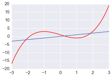
Finding fixed points
Finding the fixed points of a function \(g(x) = x\) is the same as
finding the roots of \(g(x) - x\). However, specialized algorihtms
also exist - e.g. using scipy.optimize.fixedpoint.
In [10]:
from scipy.optimize import fixed_point
In [11]:
x = np.linspace(-3,3,100)
plt.plot(x, f(x), color='red')
plt.plot(x, x)
pass
In [12]:
fixed_point(f, 0), fixed_point(f, -3), fixed_point(f, 3)
Out[12]:
(0.2541016883650524, -2.114907541476756, 1.8608058531117035)
In [13]:
newton(lambda x: f(x) - x, 0), newton(lambda x: f(x) - x, -3), newton(lambda x: f(x) - x, 3)
Out[13]:
(0.2541016883650524, -2.114907541476814, 1.8608058531117062)
In [14]:
def f(x, r):
    """Discrete logistic equation."""
    return r*x*(1-x)
In [15]:
n = 100
fps = np.zeros(n)
for i, r in enumerate(np.linspace(0, 4, n)):
    fps[i] = fixed_point(f, 0.5, args=(r, ))

plt.plot(np.linspace(0, 4, n), fps)
plt.axis([0,4,-0.1, 1.1])
pass
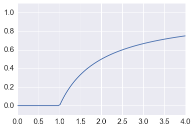
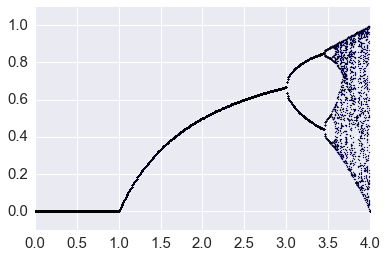
Note that we don’t know anything about the stability of the fixed point
Beyond \(r = 3\), the fixed point is unstable, even chaotic, but we would never know that just from the plot above.
In [16]:
xs = []
for i, r in enumerate(np.linspace(0, 4, 400)):
    x = 0.5
    for j in range(10000):
        x = f(x, r)
    for j in range(50):
        x = f(x, r)
        xs.append((r, x))
xs = np.array(xs)
plt.scatter(xs[:,0], xs[:,1], s=1)
plt.axis([0,4,-0.1, 1.1])
pass
Mutlivariate roots and fixed points
Use root to solve polynomial euqations. Use fsolve for
non-polynomial equations.
In [17]:
from scipy.optimize import root, fsolve
Suppose we want to solve a sysetm of \(m\) equations with \(n\) unknowns
In [18]:
def f(x):
    return [x[1] - 3*x[0]*(x[0]+1)*(x[0]-1),
            .25*x[0]**2 + x[1]**2 - 1]
In [19]:
sol = root(f, (0.5, 0.5))
sol.x
Out[19]:
array([ 1.11694147, 0.82952422])
In [20]:
fsolve(f, (0.5, 0.5))
Out[20]:
array([ 1.11694147, 0.82952422])
We can also give the jacobian
In [21]:
def jac(x):
    return [[-6*x[0], 1], [0.5*x[0], 2*x[1]]]
In [22]:
sol = root(f, (0.5, 0.5), jac=jac)
sol.x, sol.fun
Out[22]:
(array([ 1.11694147,  0.82952422]),
 array([ -4.23383550e-12,  -3.31612515e-12]))
Starting from other initial conditions, different roots may be found
In [24]:
sol = root(f, (12,12))
sol.x
Out[24]:
array([ 0.77801314, -0.92123498])
In [25]:
np.allclose(f(sol.x), 0)
Out[25]:
True
Optimization Primer
We will assume that our optimization problem is to minimize some univariate or multivariate function \(f(x)\). This is without loss of generality, since to find the maximum, we can simply minime \(-f(x)\). We will also assume that we are dealing with multivariate or real-valued smooth functions - non-smooth or discrete functions (e.g. integer-valued) are outside the scope of this course.
To find the minimum of a function, we first need to be able to express the function as a mathemtical expresssion. For example, in lesst squares regression, the function that we are optimizing is of the form \(y_i - f(x_i, \theta)\) for some parameter(s) \(\theta\). To choose an appropirate optimization algorihtm, we should at least answr these two questions if possible:
- Is the function convex?
- Are there any constraints that the solution must meet?
Finally, we need to realize that optimization mehthods are nearly always designed to find local optima. For convex problems, there is only one minimum and so this is not a problem. However, if there are multiple local minima, often heuristics such as multiple random starts must be adopted to find a “good” enouhg solution.
Is the function convex?
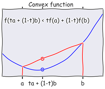
Convex functions are very nice because they have a single global minimum, and there are very efficient algorithms for solving large convex systems.
Intuitively, a function is convex if every chord joining two points on the function lies above the function. More formally, a function is convex if
for some \(t\) between 0 and 1 - this is shown in the figure below.
In [26]:
def f(x):
    return (x-4)**2 + x + 1

with plt.xkcd():
    x = np.linspace(0, 10, 100)

    plt.plot(x, f(x))
    ymin, ymax = plt.ylim()
    plt.axvline(2, ymin, f(2)/ymax, c='red')
    plt.axvline(8, ymin, f(8)/ymax, c='red')
    plt.scatter([4, 4], [f(4), f(2) + ((4-2)/(8-2.))*(f(8)-f(2))],
                 edgecolor=['blue', 'red'], facecolor='none', s=100, linewidth=2)
    plt.plot([2,8], [f(2), f(8)])
    plt.xticks([2,4,8], ('a', 'ta + (1-t)b', 'b'), fontsize=20)
    plt.text(0.2, 40, 'f(ta + (1-t)b) < tf(a) + (1-t)f(b)', fontsize=20)
    plt.xlim([0,10])
    plt.yticks([])
    plt.suptitle('Convex function', fontsize=20)
Warm up exercise
Show that \(f(x) = -\log(x)\) is a convex function.
Checking if a function is convex using the Hessian
The formal definition is only useful for checking if a function is convex if you can find a counter-example. More practically, a twice differentiable function is convex if its Hessian is positive semi-definite, and strictly convex if the Hessian is positive definite.
For example, suppose we want to minimize the scalar-valued function
In [27]:
from sympy import symbols, hessian, Function, init_printing, expand, Matrix, diff
x, y, z = symbols('x y z')
f = symbols('f', cls=Function)
init_printing()
In [28]:
f = x**2 + 2*y**2 + 3*z**2 + 2*x*y + 2*x*z
f
Out[28]:
In [29]:
H = hessian(f, (x, y, z))
H
Out[29]:
In [30]:
np.real_if_close(la.eigvals(np.array(H).astype('float')))
Out[30]:
array([ 0.24122952, 7.06417777, 4.69459271])
Since the matrix is symmetric and all eigenvalues are positive, the Hessian is positive defintie and the function is convex.
Combining convex functions
The following rules may be useful to determine if more complex functions are covex:
- The intersection of convex functions is convex
- If the functions \(f\) and \(g\) are convex and \(a \ge 0\) and \(b \ge 0\) then the function \(af + bg\) is convex.
- If the function \(U\) is convex and the function \(g\) is nondecreasing and convex then the function f defined by \(f (x) = g(U(x))\) is convex.
Many more technical deetails about convexity and convex optimization can be found in this book.
Are there any constraints that the solution must meet?
In general, optimizaiton without constraints is easier to solve than optimization in the presence of constraints. In any case, the solutions may be very different in the prsence or absence of constraints, so it is important to know if there are any constraints.
We will see some examples of two general strategies - convert a problme with constraints into one without constraints, or use an algorithm that can optimize with constraints.
Using scipy.optimize
One of the most convenient libraries to use is scipy.optimize, since
it is already part of the Anaconda installation and it has a fairly
intuitive interface.
In [31]:
from scipy import optimize as opt
In [32]:
def f(x):
    return x**4 + 3*(x-2)**3 - 15*(x)**2 + 1
In [33]:
x = np.linspace(-8, 5, 100)
plt.plot(x, f(x));
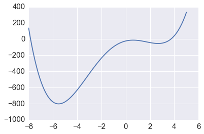
The
`minimize_scalar <http://docs.scipy.org/doc/scipy/reference/generated/scipy.optimize.minimize_scalar.html#scipy.optimize.minimize_scalar>`__
function will find the minimum, and can also be told to search within
given bounds. By default, it uses the Brent algorithm, which combines a
bracketing strategy with a parabolic approximation.
In [34]:
opt.minimize_scalar(f, method='Brent')
Out[34]:
nit: 11
 nfev: 12
    x: -5.5288011252196627
  fun: -803.39553088258845
In [35]:
opt.minimize_scalar(f, method='bounded', bounds=[0, 6])
Out[35]:
nfev: 12
 success: True
     fun: -54.210039377127622
  status: 0
 message: 'Solution found.'
       x: 2.6688651040396532
Local and global minima
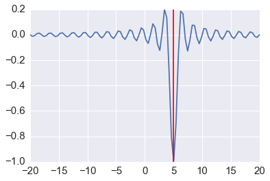
In [36]:
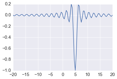
def f(x, offset):
    return -np.sinc(x-offset)
In [37]:
x = np.linspace(-20, 20, 100)
plt.plot(x, f(x, 5));
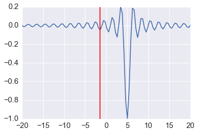
In [38]:
# note how additional function arguments are passed in
sol = opt.minimize_scalar(f, args=(5,))
sol
Out[38]:
nit: 10
 nfev: 11
    x: -1.4843871263953001
  fun: -0.049029624014074166
In [39]:
plt.plot(x, f(x, 5))
plt.axvline(sol.x, c='red')
pass
We can try multiple ranodm starts to find the global minimum
In [40]:
lower = np.random.uniform(-20, 20, 100)
upper = lower + 1
sols = [opt.minimize_scalar(f, args=(5,), bracket=(l, u)) for (l, u) in zip(lower, upper)]
In [41]:
idx = np.argmin([sol.fun for sol in sols])
sol = sols[idx]
In [42]:
plt.plot(x, f(x, 5))
plt.axvline(sol.x, c='red');

Using a stochastic algorithm
See documentation for the
`basinhopping <http://docs.scipy.org/doc/scipy-0.14.0/reference/generated/scipy.optimize.basinhopping.html>`__
algorithm, which also works with multivariate scalar optimization. Note
that this is heuristic and not guaranteed to find a global minimum.
In [43]:
from scipy.optimize import basinhopping

x0 = 0
sol = basinhopping(f, x0, stepsize=1, minimizer_kwargs={'args': (5,)})
sol
Out[43]:
nfev: 1812
                  njev: 604
                   fun: -1.0
                   nit: 100
               message: ['requested number of basinhopping iterations completed successfully']
                     x: array([ 5.])
 minimization_failures: 0
In [44]:
plt.plot(x, f(x, 5))
plt.axvline(sol.x, c='red');
Minimizing a multivariate function \(f: \mathbb{R}^n \rightarrow \mathbb{R}\)
We will next move on to optimization of multivariate scalar functions, where the scalar may (say) be the norm of a vector. Minimizing a multivariable set of equations \(f: \mathbb{R}^n \rightarrow \mathbb{R}\)^n$ is not well-defined, but we will later see how to solve the closely related problme of finding roots or fixed points of such a set of equations.
We will use the Rosenbrock “banana” function to illustrate unconstrained multivariate optimization. In 2D, this is
The function has a global minimum at (1,1) and the standard expression takes \(a = 1\) and \(b = 100\).
Conditioning of optimization problem
With these values fr \(a\) and \(b\), the problem is ill-conditioned. As we shall see, one of the factors affecting the ease of optimization is the condition number of the curvature (Hessian). When the condition number is high, the gradient may not point in the direction of the minimum, and simple gradient descent methods may be inefficient since they may be forced to take many sharp turns.
In [45]:
from sympy import symbols, hessian, Function, N

x, y = symbols('x y')
f = symbols('f', cls=Function)

f = 100*(y - x**2)**2 + (1 - x)**2

H = hessian(f, [x, y]).subs([(x,1), (y,1)])
H, N(H.condition_number())
Out[45]:
As pointed out in the previous lecture, the condition number is basically the ratio of largest to smallest eigenvalue of the Hessian
In [46]:
import scipy.linalg as la

mu = la.eigvals(np.array([802, -400, -400, 200]).reshape((2,2)))
np.real_if_close(mu[0]/mu[1])
Out[46]:
array(2508.009601277337)
In [47]:
def rosen(x):
    """Generalized n-dimensional version of the Rosenbrock function"""
    return sum(100*(x[1:]-x[:-1]**2.0)**2.0 +(1-x[:-1])**2.0)
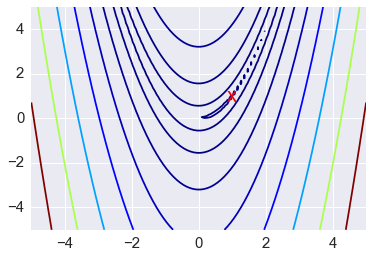
Why is the condition number so large?
In [48]:
x = np.linspace(-5, 5, 100)
y = np.linspace(-5, 5, 100)
X, Y = np.meshgrid(x, y)
Z = rosen(np.vstack([X.ravel(), Y.ravel()])).reshape((100,100))
In [49]:
# Note: the global minimum is at (1,1) in a tiny contour island
plt.contour(X, Y, Z, np.arange(10)**5, cmap='jet')
plt.text(1, 1, 'x', va='center', ha='center', color='red', fontsize=20);
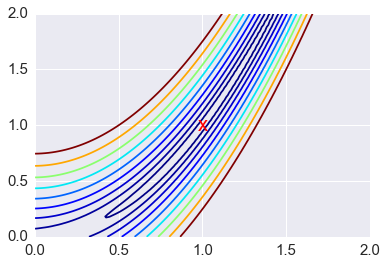
Zooming in to the global minimum at (1,1)
In [50]:
x = np.linspace(0, 2, 100)
y = np.linspace(0, 2, 100)
X, Y = np.meshgrid(x, y)
Z = rosen(np.vstack([X.ravel(), Y.ravel()])).reshape((100,100))
In [51]:
plt.contour(X, Y, Z, [rosen(np.array([k, k])) for k in np.linspace(1, 1.5, 10)], cmap='jet')
plt.text(1, 1, 'x', va='center', ha='center', color='red', fontsize=20);
Gradient descent
The gradient (or Jacobian) at a point indicates the direction of steepest ascent. Since we are looking for a minimum, one obvious possibility is to take a step in the opposite direction to the gradient. We weight the size of the step by a factor \(\alpha\) known in the machine learning literature as the learning rate. If \(\alpha\) is small, the algorithm will eventually converge towards a local minimum, but it may take long time. If \(\alpha\) is large, the algorithm may converge faster, but it may also overshoot and never find the minimum. Gradient descent is also known as a first order method because it requires calculation of the first derivative at each iteration.
Some algorithms also determine the appropriate value of \(\alpha\) at each stage by using a line search, i.e.,
which is a 1D optimization problem.
As suggested above, the problem is that the gradient may not point towards the global minimum especially when the condition number is large, and we are forced to use a small \(\alpha\) for convergence.
Let’s warm up by minimizing a trivial function \(f(x, y) = x^2 + y^2\) to illustrate the basic idea of gradient descent.
In [54]:
def f(x):
    return x[0]**2 + x[1]**2

def grad(x):
    return np.array([2*x[0], 2*x[1]])

a = 0.1 # learning rate
x0 = np.array([1.0,1.0])
print('Start', x0)
for i in range(41):
    x0 -= a * grad(x0)
    if i%5 == 0:
        print(i, x0)
Start [ 1.  1.]
0 [ 0.8  0.8]
5 [ 0.262144  0.262144]
10 [ 0.08589935  0.08589935]
15 [ 0.0281475  0.0281475]
20 [ 0.00922337  0.00922337]
25 [ 0.00302231  0.00302231]
30 [ 0.00099035  0.00099035]
35 [ 0.00032452  0.00032452]
40 [ 0.00010634  0.00010634]
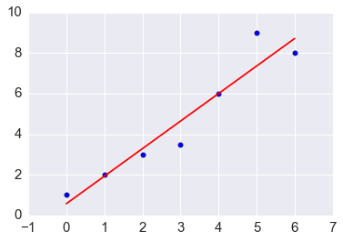
Gradient descent for least squares minimization
Usually, when we optimize, we are not just finding the minimum, but also want to know the parameters that give us the minimum. As a simple example, suppose we want to find parameters that minimize the least squares difference between a linear model and some data. Suppose we have some data \((0,1), (1,2), (2,3), (3,3.5), (4,6), (5,9), (6,8)\) and want to find a line \(y = \beta_0 +\beta_1 x\) that is the best least squares fit. One way to do this is to solve \(X^TX\hat{\beta} = X^Ty\), but we want to show how this can be formulated as a gradient descent problem.
We want to find \(\beta = (\beta_0, \beta_1)\) that minimize the squared differences
We calculate the gradient with respect to \(\beta\) as
and apply gradient descent.
In [13]:
def f(x, y, b):
    """Helper function."""
    return (b[0] + b[1]*x - y)

def grad(x, y, b):
    """Gradient of objective function with respect to parameters b."""
    n = len(x)
    return np.array([
            sum(f(x, y, b)),
            sum(x*f(x, y, b))
    ])
In [10]:
x, y = map(np.array, zip((0,1), (1,2), (2,3), (3,3.5), (4,6), (5,9), (6,8)))
In [16]:
a = 0.001 # learning rate
b0 = np.zeros(2)
for i in range(10000):
    b0 -= a * grad(x, y, b0)
In [17]:
plt.scatter(x, y, s=30)
plt.plot(x, b0[0] + b0[1]*x, color='red')
pass
Gradient descent to minimize the Rosen function using scipy.optimize
Because gradient descent is unreliable in practice, it is not part of
the scipy optimize suite of functions, but we will write a custom
function below to illustrate how to use gradient descent while
maintaining the scipy.optimize interface.
In [52]:
def rosen_der(x):
    """Derivative of generalized Rosen function."""
    xm = x[1:-1]
    xm_m1 = x[:-2]
    xm_p1 = x[2:]
    der = np.zeros_like(x)
    der[1:-1] = 200*(xm-xm_m1**2) - 400*(xm_p1 - xm**2)*xm - 2*(1-xm)
    der[0] = -400*x[0]*(x[1]-x[0]**2) - 2*(1-x[0])
    der[-1] = 200*(x[-1]-x[-2]**2)
    return der
Warning One of the most common causes of failure of optimization is
because the gradient or Hessian function is specified incorrectly. You
can check for this using check_grad which compares the analytical
gradient with one calculated using finite differences.
In [53]:
from scipy.optimize import check_grad

for x in np.random.uniform(-2,2,(10,2)):
    x0 = np.array(x)
    print(x0, check_grad(rosen, rosen_der, x0))
[ 0.84795961  0.8841431 ] 4.12099762158e-06
[ 0.25702089  1.12043717] 2.22491327726e-06
[ 1.06226702 -1.80970275] 3.12407324679e-05
[ 1.5334192 -1.5059954] 1.13208298556e-05
[-0.15930274  1.80868951] 3.71611303963e-06
[ 1.32643444 -1.18424149] 3.25553261955e-05
[ 0.49184844 -0.00341954] 2.67781137655e-06
[ 0.85557139  1.12996825] 3.31235322885e-06
[-1.00825153 -1.85587153] 1.62466187316e-05
[ 0.41514196  0.6850504 ] 1.7634932791e-06
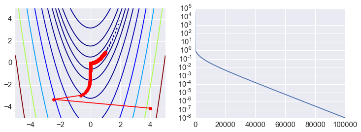
Writing a custom function for the scipy.optimize interface.
In [55]:
def custmin(fun, x0, args=(), maxfev=None, alpha=0.0002,
        maxiter=100000, tol=1e-10, callback=None, **options):
    """Implements simple gradient descent for the Rosen function."""
    bestx = x0
    besty = fun(x0)
    funcalls = 1
    niter = 0
    improved = True
    stop = False

    while improved and not stop and niter < maxiter:
        niter += 1
        # the next 2 lines are gradient descent
        step = alpha * rosen_der(bestx)
        bestx = bestx - step

        besty = fun(bestx)
        funcalls += 1

        if la.norm(step) < tol:
            improved = False
        if callback is not None:
            callback(bestx)
        if maxfev is not None and funcalls >= maxfev:
            stop = True
            break

    return opt.OptimizeResult(fun=besty, x=bestx, nit=niter,
                              nfev=funcalls, success=(niter > 1))
In [56]:
def reporter(p):
    """Reporter function to capture intermediate states of optimization."""
    global ps
    ps.append(p)
In [57]:
# Initial starting position
x0 = np.array([4,-4.1])
In [58]:
ps = [x0]
opt.minimize(rosen, x0, method=custmin, callback=reporter)
Out[58]:
nit: 100000
 success: True
    nfev: 100001
       x: array([ 0.9998971 ,  0.99979381])
     fun: 1.0604663473448339e-08
In [59]:
x = np.linspace(-5, 5, 100)
y = np.linspace(-5, 5, 100)
X, Y = np.meshgrid(x, y)
Z = rosen(np.vstack([X.ravel(), Y.ravel()])).reshape((100,100))
In [60]:
ps = np.array(ps)
plt.figure(figsize=(12,4))
plt.subplot(121)
plt.contour(X, Y, Z, np.arange(10)**5, cmap='jet')
plt.plot(ps[:, 0], ps[:, 1], '-ro')
plt.subplot(122)
plt.semilogy(range(len(ps)), rosen(ps.T));
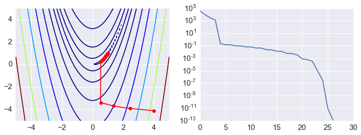
Newton’s method and variants
Recall Newton’s method for finding roots of a univariate function
When we are looking for a minimum, we are looking for the roots of the derivative \(f'(x)\), so
Newotn’s method can also be seen as a Taylor series approximation
At the function minimum, the derivtive is 0, so
and letting \(\Delta x = \frac{h}{2}\), we get that the Newton stpe is
The multivariate analog replaces \(f'\) with the Jacobian and \(f''\) with the Hessian, so the Newton step is
Second order methods
Second order methods solve for \(H^{-1}\) and so require calculation
of the Hessian (either provided or approximated using finite
differences). For efficiency reasons, the Hessian is not directly
inverted, but solved for using a variety of methods such as conjugate
gradient. An example of a second order method in the optimize
package is Newton-GC.
In [61]:
from scipy.optimize import rosen, rosen_der, rosen_hess
In [62]:
ps = [x0]
opt.minimize(rosen, x0, method='Newton-CG', jac=rosen_der, hess=rosen_hess, callback=reporter)
Out[62]:
success: True
    nfev: 38
     fun: 1.3642782750354208e-13
     nit: 26
    njev: 63
    nhev: 26
  status: 0
 message: 'Optimization terminated successfully.'
       x: array([ 0.99999963,  0.99999926])
     jac: array([  1.21204353e-04,  -6.08502470e-05])
In [63]:
ps = np.array(ps)
plt.figure(figsize=(12,4))
plt.subplot(121)
plt.contour(X, Y, Z, np.arange(10)**5, cmap='jet')
plt.plot(ps[:, 0], ps[:, 1], '-ro')
plt.subplot(122)
plt.semilogy(range(len(ps)), rosen(ps.T));
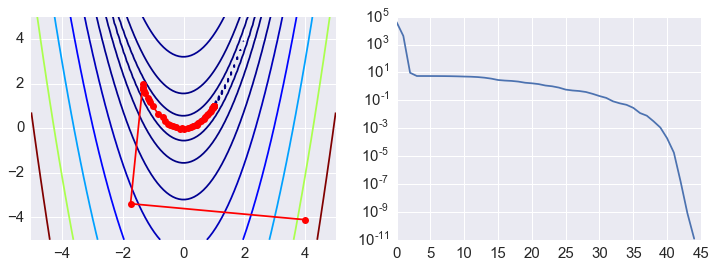
Frist order methods
As calculating the Hessian is computationally expensive, first order
methods only use the first derivatives. Quasi-Newton methods use
functions of the first derivatives to approximate the inverse Hessian. A
well know example of the Quasi-Newoton class of algorithjms is BFGS,
named after the initials of the creators. As usual, the first
derivatives can either be provided via the jac= argument or
approximated by finite difference methods.
In [64]:
ps = [x0]
opt.minimize(rosen, x0, method='BFGS', callback=reporter)
Out[64]:
nfev: 280
 hess_inv: array([[ 0.49982388,  0.99958969],
       [ 0.99958969,  2.00405492]])
      fun: 1.2055799758407391e-11
      nit: 44
     njev: 67
  success: False
   status: 2
  message: 'Desired error not necessarily achieved due to precision loss.'
        x: array([ 0.99999659,  0.99999311])
      jac: array([  2.46198954e-05,  -1.12454678e-05])
In [65]:
ps = np.array(ps)
plt.figure(figsize=(12,4))
plt.subplot(121)
plt.contour(X, Y, Z, np.arange(10)**5, cmap='jet')
plt.plot(ps[:, 0], ps[:, 1], '-ro')
plt.subplot(122)
plt.semilogy(range(len(ps)), rosen(ps.T));
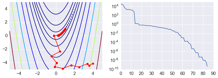
Zeroth order methods
Finally, there are some optimization algorithms not based on the Newton method, but on other heuristic search strategies that do not require any derivatives, only function evaluations. One well-known example is the Nelder-Mead simplex algorithm.
In [66]:
ps = [x0]
opt.minimize(rosen, x0, method='nelder-mead', callback=reporter)
Out[66]:
nfev: 162
 success: True
  status: 0
     fun: 5.262756878429089e-10
     nit: 85
 message: 'Optimization terminated successfully.'
       x: array([ 0.99998846,  0.99997494])
In [67]:
ps = np.array(ps)
plt.figure(figsize=(12,4))
plt.subplot(121)
plt.contour(X, Y, Z, np.arange(10)**5, cmap='jet')
plt.plot(ps[:, 0], ps[:, 1], '-ro')
plt.subplot(122)
plt.semilogy(range(len(ps)), rosen(ps.T));
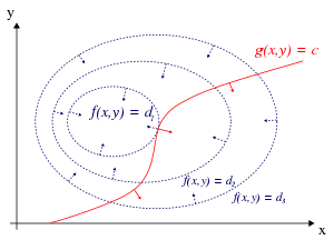
Lagrange multipliers and constrained optimization
Recall why Lagrange multipliers are useful for constrained optimization - a stationary point must be where the constraint surface \(g\) touches a level set of the function \(f\) (since the value of \(f\) does not change on a level set). At that point, \(f\) and \(g\) are parallel, and hence their gradients are also parallel (since the gradient is normal to the level set). So we want to solve
or equivalently,
Lagrange multipliers
Numerical example of using Lagrange multipliers
Maximize \(f (x, y, z) = xy + yz\) subject to the constraints \(x + 2y = 6\) and \(x − 3z = 0\).
We set up the equations
Now set partial derivatives to zero and solve the following set of equations
which is a linear equation in \(x, y, z, \lambda, \mu\)
In [68]:
A = np.array([
    [0, 1, 0, -1, -1],
    [1, 0, 1, -2, 0],
    [0, 1, 0, 0, 3],
    [1, 2, 0, 0, 0],
    [1, 0,-3, 0, 0]])

b = np.array([0,0,0,6,0])

sol = la.solve(A, b)
In [69]:
sol
Out[69]:
array([ 3. , 1.5, 1. , 2. , -0.5])
In [70]:
def f(x, y, z):
    return x*y + y*z
In [71]:
f(*sol[:3])
Out[71]:
Check using scipy.optimize
In [72]:
# Convert to minimization problem by negating function
def f(x):
    return -(x[0]*x[1] + x[1]*x[2])
In [73]:
cons = ({'type': 'eq',
         'fun' : lambda x: np.array([x[0] + 2*x[1] - 6, x[0] - 3*x[2]])})
In [74]:
x0 = np.array([2,2,0.67])
cx = opt.minimize(f, x0, constraints=cons)
cx
Out[74]:
nfev: 15
     fun: -5.9999999999999689
     nit: 3
    njev: 3
 success: True
  status: 0
 message: 'Optimization terminated successfully.'
       x: array([ 2.99999979,  1.50000011,  0.99999993])
     jac: array([-1.50000012, -3.9999997 , -1.50000012,  0.        ])
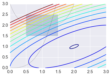
Another example of constrained optimization
Many real-world optimization problems have constraints - for example, a set of parameters may have to sum to 1.0 (equality constraint), or some parameters may have to be non-negative (inequality constraint). Sometimes, the constraints can be incorporated into the function to be minimized, for example, the non-negativity constraint \(p \gt 0\) can be removed by substituting \(p = e^q\) and optimizing for \(q\). Using such workarounds, it may be possible to convert a constrained optimization problem into an unconstrained one, and use the methods discussed above to solve the problem.
Alternatively, we can use optimization methods that allow the specification of constraints directly in the problem statement as shown in this section. Internally, constraint violation penalties, barriers and Lagrange multipliers are some of the methods used used to handle these constraints. We use the example provided in the Scipy tutorial to illustrate how to set constraints.
subject to the constraint
and the bounds
In [75]:
def f(x):
    return -(2*x[0]*x[1] + 2*x[0] - x[0]**2 - 2*x[1]**2)
In [76]:
x = np.linspace(0, 3, 100)
y = np.linspace(0, 3, 100)
X, Y = np.meshgrid(x, y)
Z = f(np.vstack([X.ravel(), Y.ravel()])).reshape((100,100))
plt.contour(X, Y, Z, np.arange(-1.99,10, 1), cmap='jet');
plt.plot(x, x**3, 'k:', linewidth=1)
plt.plot(x, (x-1)**4+2, 'k:', linewidth=1)
plt.fill([0.5,0.5,1.5,1.5], [2.5,1.5,1.5,2.5], alpha=0.3)
plt.axis([0,3,0,3])
Out[76]:
To set constraints, we pass in a dictionary with keys ty;pe, fun
and jac. Note that the inequality constraint assumes a
\(C_j x \ge 0\) form. As usual, the jac is optional and will be
numerically estimate if not provided.
In [77]:
cons = ({'type': 'eq',
         'fun' : lambda x: np.array([x[0]**3 - x[1]]),
         'jac' : lambda x: np.array([3.0*(x[0]**2.0), -1.0])},
        {'type': 'ineq',
         'fun' : lambda x: np.array([x[1] - (x[0]-1)**4 - 2])})

bnds = ((0.5, 1.5), (1.5, 2.5))
In [78]:
x0 = [0, 2.5]
Unconstrained optimization
In [79]:
ux = opt.minimize(f, x0, constraints=None)
ux
Out[79]:
nfev: 20
 hess_inv: array([[ 0.99999996,  0.49999996],
       [ 0.49999996,  0.49999997]])
      fun: -1.9999999999999987
      nit: 3
     njev: 5
  success: True
   status: 0
  message: 'Optimization terminated successfully.'
        x: array([ 1.99999996,  0.99999996])
      jac: array([ 0.,  0.])
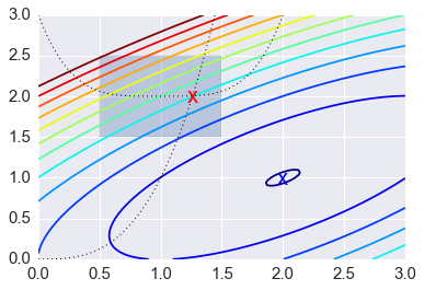
Constrained optimization
In [80]:
cx = opt.minimize(f, x0, bounds=bnds, constraints=cons)
cx
Out[80]:
nfev: 21
     fun: 2.0499154720925521
     nit: 5
    njev: 5
 success: True
  status: 0
 message: 'Optimization terminated successfully.'
       x: array([ 1.26089314,  2.00463288])
     jac: array([-3.48747873,  5.49674428,  0.        ])
In [81]:
x = np.linspace(0, 3, 100)
y = np.linspace(0, 3, 100)
X, Y = np.meshgrid(x, y)
Z = f(np.vstack([X.ravel(), Y.ravel()])).reshape((100,100))
plt.contour(X, Y, Z, np.arange(-1.99,10, 1), cmap='jet');
plt.plot(x, x**3, 'k:', linewidth=1)
plt.plot(x, (x-1)**4+2, 'k:', linewidth=1)
plt.text(ux['x'][0], ux['x'][1], 'x', va='center', ha='center', size=20, color='blue')
plt.text(cx['x'][0], cx['x'][1], 'x', va='center', ha='center', size=20, color='red')
plt.fill([0.5,0.5,1.5,1.5], [2.5,1.5,1.5,2.5], alpha=0.3)
plt.axis([0,3,0,3]);
Some applications of optimization
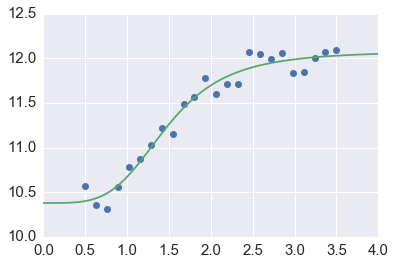
Curve fitting
Sometimes, we simply want to use non-linear least squares to fit a
function to data, perhaps to estimate parameters for a mechanistic or
phenomenological model. The curve_fit function uses the quasi-Newton
Levenberg-Marquadt algorithm to perform such fits. Behind the scenes,
curve_fit is just a wrapper around the leastsq function that
does nonlinear least squares fitting.
In [82]:
from scipy.optimize import curve_fit
In [83]:
def logistic4(x, a, b, c, d):
    """The four paramter logistic function is often used to fit dose-response relationships."""
    return ((a-d)/(1.0+((x/c)**b))) + d
In [84]:
nobs = 24
xdata = np.linspace(0.5, 3.5, nobs)
ptrue = [10, 3, 1.5, 12]
ydata = logistic4(xdata, *ptrue) + 0.5*np.random.random(nobs)
In [85]:
popt, pcov = curve_fit(logistic4, xdata, ydata)
In [86]:
perr = yerr=np.sqrt(np.diag(pcov))
print('Param\tTrue\tEstim (+/- 1 SD)')
for p, pt, po, pe  in zip('abcd', ptrue, popt, perr):
    print('%s\t%5.2f\t%5.2f (+/-%5.2f)' % (p, pt, po, pe))
Param   True    Estim (+/- 1 SD)
a       10.00   10.38 (+/- 0.09)
b        3.00    4.04 (+/- 0.77)
c        1.50    1.47 (+/- 0.07)
d       12.00   12.08 (+/- 0.08)
In [87]:
x = np.linspace(0, 4, 100)
y = logistic4(x, *popt)
plt.plot(xdata, ydata, 'o')
plt.plot(x, y);
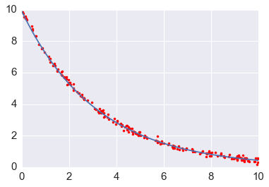
Finding paraemeters for ODE models
This is a specialized application of curve_fit, in which the curve
to be fitted is defined implicitly by an ordinary differential equation
and we want to use observed data to estimate the parameters \(k\) and the initial value \(x_0\). Of course this can be explicitly solved but the same approach can be used to find multiple parameters for \(n\)-dimensional systems of ODEs.
A more elaborate example for fitting a system of ODEs to model the zombie apocalypse
In [88]:
from scipy.integrate import odeint

def f(x, t, k):
    """Simple exponential decay."""
    return -k*x

def x(t, k, x0):
    """
    Solution to the ODE x'(t) = f(t,x,k) with initial condition x(0) = x0
    """
    x = odeint(f, x0, t, args=(k,))
    return x.ravel()
In [89]:
# True parameter values
x0_ = 10
k_ = 0.1*np.pi

# Some random data genererated from closed form soltuion plus Gaussian noise
ts = np.sort(np.random.uniform(0, 10, 200))
xs = x0_*np.exp(-k_*ts) + np.random.normal(0,0.1,200)

popt, cov = curve_fit(x, ts, xs)
k_opt, x0_opt = popt

print("k = %g" % k_opt)
print("x0 = %g" % x0_opt)
k = 0.313004
x0 = 9.88547
In [90]:
import matplotlib.pyplot as plt
t = np.linspace(0, 10, 100)
plt.plot(ts, xs, 'r.', t, x(t, k_opt, x0_opt), '-');
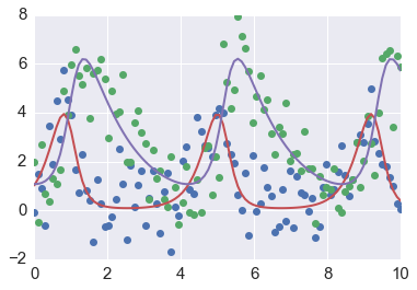
Another example of fitting a system of ODEs using the lmfit package
You may have to install the
`lmfit <http://cars9.uchicago.edu/software/python/lmfit/index.html>`__
package using pip and restart your kernel. The lmfit algorithm
is another wrapper around scipy.optimize.leastsq but allows for
richer model specification and more diagnostics.
In [91]:
from lmfit import minimize, Parameters, Parameter, report_fit
import warnings
In [92]:
def f(xs, t, ps):
    """Lotka-Volterra predator-prey model."""
    try:
        a = ps['a'].value
        b = ps['b'].value
        c = ps['c'].value
        d = ps['d'].value
    except:
        a, b, c, d = ps

    x, y = xs
    return [a*x - b*x*y, c*x*y - d*y]

def g(t, x0, ps):
    """
    Solution to the ODE x'(t) = f(t,x,k) with initial condition x(0) = x0
    """
    x = odeint(f, x0, t, args=(ps,))
    return x

def residual(ps, ts, data):
    x0 = ps['x0'].value, ps['y0'].value
    model = g(ts, x0, ps)
    return (model - data).ravel()

t = np.linspace(0, 10, 100)
x0 = np.array([1,1])

a, b, c, d = 3,1,1,1
true_params = np.array((a, b, c, d))

np.random.seed(123)
data = g(t, x0, true_params)
data += np.random.normal(size=data.shape)

# set parameters incluing bounds
params = Parameters()
params.add('x0', value= float(data[0, 0]), min=0, max=10)
params.add('y0', value=float(data[0, 1]), min=0, max=10)
params.add('a', value=2.0, min=0, max=10)
params.add('b', value=2.0, min=0, max=10)
params.add('c', value=2.0, min=0, max=10)
params.add('d', value=2.0, min=0, max=10)

# fit model and find predicted values
result = minimize(residual, params, args=(t, data), method='leastsq')
final = data + result.residual.reshape(data.shape)

# plot data and fitted curves
plt.plot(t, data, 'o')
plt.plot(t, final, '-', linewidth=2);

# display fitted statistics
report_fit(result)
[[Fit Statistics]]
    # function evals   = 169
    # data points      = 200
    # variables        = 6
    chi-square         = 212.716
    reduced chi-square = 1.096
[[Variables]]
    x0:   1.02052198 +/- 0.181683 (17.80%) (init= 0)
    y0:   1.07046508 +/- 0.110177 (10.29%) (init= 1.997345)
    a:    3.54341848 +/- 0.454160 (12.82%) (init= 2)
    b:    1.21280681 +/- 0.148475 (12.24%) (init= 2)
    c:    0.84529664 +/- 0.079478 (9.40%) (init= 2)
    d:    0.85715536 +/- 0.085627 (9.99%) (init= 2)
[[Correlations]] (unreported correlations are <  0.100)
    C(a, b)                      =  0.960
    C(a, d)                      = -0.956
    C(b, d)                      = -0.878
    C(x0, b)                     = -0.759
    C(x0, a)                     = -0.745
    C(y0, c)                     = -0.717
    C(y0, d)                     = -0.683
    C(c, d)                      =  0.667
    C(x0, d)                     =  0.578
    C(a, c)                      = -0.532
    C(y0, a)                     =  0.475
    C(b, c)                      = -0.433
    C(y0, b)                     =  0.271
/Users/cliburn/anaconda/envs/py35/lib/python3.5/site-packages/ipykernel/__main__.py:4: DeprecationWarning: using a non-integer number instead of an integer will result in an error in the future
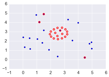
Optimization of graph node placement
To show the many different applications of optimization, here is an example using optimization to change the layout of nodes of a graph. We use a physical analogy - nodes are connected by springs, and the springs resist deformation from their natural length \(l_{ij}\). Some nodes are pinned to their initial locations while others are free to move. Because the initial configuration of nodes does not have springs at their natural length, there is tension resulting in a high potential energy \(U\), given by the physics formula shown below. Optimization finds the configuration of lowest potential energy given that some nodes are fixed (set up as boundary constraints on the positions of the nodes).
Note that the ordination algorithm Multi-Dimensional Scaling (MDS) works on a very similar idea - take a high dimensional data set in \(\mathbb{R}^n\), and project down to a lower dimension (\(\mathbb{R}^k\)) such that the sum of distances \(d_n(x_i, x_j) - d_k(x_i, x_j)\), where \(d_n\) and \(d_k\) are some measure of distance between two points \(x_i\) and \(x_j\) in \(n\) and \(d\) dimension respectively, is minimized. MDS is often used in exploratory analysis of high-dimensional data to get some intuitive understanding of its “structure”.
In [93]:
from scipy.spatial.distance import pdist, squareform
- P0 is the initial location of nodes
- P is the minimal energy location of nodes given constraints
- A is a connectivity matrix - there is a spring between \(i\) and \(j\) if \(A_{ij} = 1\)
- \(L_{ij}\) is the resting length of the spring connecting \(i\) and \(j\)
- In addition, there are a number of
fixednodes whose positions are pinned.
In [94]:
n = 20
k = 1 # spring stiffness
P0 = np.random.uniform(0, 5, (n,2))
A = np.ones((n, n))
A[np.tril_indices_from(A)] = 0
L = A.copy()
In [95]:
def energy(P):
    P = P.reshape((-1, 2))
    D = squareform(pdist(P))
    return 0.5*(k * A * (D - L)**2).sum()
In [96]:
energy(P0.ravel())
Out[96]:
In [97]:
# fix the position of the first few nodes just to show constraints
fixed = 4
bounds = (np.repeat(P0[:fixed,:].ravel(), 2).reshape((-1,2)).tolist() +
          [[None, None]] * (2*(n-fixed)))
bounds[:fixed*2+4]
Out[97]:
[[1.191249528562059, 1.191249528562059],
 [4.0389554314507805, 4.0389554314507805],
 [4.474891439430058, 4.474891439430058],
 [0.216114460398234, 0.216114460398234],
 [1.5097341813135952, 1.5097341813135952],
 [4.902910992971438, 4.902910992971438],
 [2.6975241127686767, 2.6975241127686767],
 [3.1315468085492815, 3.1315468085492815],
 [None, None],
 [None, None],
 [None, None],
 [None, None]]
In [98]:
sol = opt.minimize(energy, P0.ravel(), bounds=bounds)
Visualization
Original placement is BLUE Optimized arrangement is RED.
In [99]:
plt.scatter(P0[:, 0], P0[:, 1], s=25)
P = sol.x.reshape((-1,2))
plt.scatter(P[:, 0], P[:, 1], edgecolors='red', facecolors='none', s=30, linewidth=2);
Optimization of standard statistical models
When we solve standard statistical problems, an optimization procedure similar to the ones discussed here is performed. For example, consider multivariate logistic regression - typically, a Newton-like algorithm known as iteratively reweighted least squares (IRLS) is used to find the maximum likelihood estimate for the generalized linear model family. However, using one of the multivariate scalar minimization methods shown above will also work, for example, the BFGS minimization algorithm.
The take home message is that there is nothing magic going on when Python or R fits a statistical model using a formula - all that is happening is that the objective function is set to be the negative of the log likelihood, and the minimum found using some first or second order optimization algorithm.
In [100]:
import statsmodels.api as sm
Logistic regression as optimization
Suppose we have a binary outcome measure \(Y \in {0,1}\) that is conditinal on some input variable (vector) \(x \in (-\infty, +\infty)\). Let the conditioanl probability be \(p(x) = P(Y=y | X=x)\). Given some data, one simple probability model is \(p(x) = \beta_0 + x\cdot\beta\) - i.e. linear regression. This doesn’t really work for the obvious reason that \(p(x)\) must be between 0 and 1 as \(x\) ranges across the real line. One simple way to fix this is to use the transformation \(g(x) = \frac{p(x)}{1 - p(x)} = \beta_0 + x.\beta\). Solving for \(p\), we get
As you all know very well, this is logistic regression.
Suppose we have \(n\) data points \((x_i, y_i)\) where \(x_i\) is a vector of features and \(y_i\) is an observed class (0 or 1). For each event, we either have “success” (\(y = 1\)) or “failure” (\(Y = 0\)), so the likelihood looks like the product of Bernoulli random variables. According to the logistic model, the probability of success is \(p(x_i)\) if \(y_i = 1\) and \(1-p(x_i)\) if \(y_i = 0\). So the likelihood is
and the log-likelihood is
Using the standard ‘trick’, if we augment the matrix \(X\) with a column of 1s, we can write \(\beta_0 + x_i\cdot\beta\) as just \(X\beta\).
In [101]:
df_ = pd.read_csv("http://www.ats.ucla.edu/stat/data/binary.csv")
df_.head()
Out[101]:
| admit | gre | gpa | rank | |
|---|---|---|---|---|
| 0 | 0 | 380 | 3.61 | 3 |
| 1 | 1 | 660 | 3.67 | 3 |
| 2 | 1 | 800 | 4.00 | 1 |
| 3 | 1 | 640 | 3.19 | 4 |
| 4 | 0 | 520 | 2.93 | 4 |
In [102]:
# We will ignore the rank categorical value

cols_to_keep = ['admit', 'gre', 'gpa']
df = df_[cols_to_keep]
df.insert(1, 'dummy', 1)
df.head()
Out[102]:
| admit | dummy | gre | gpa | |
|---|---|---|---|---|
| 0 | 0 | 1 | 380 | 3.61 |
| 1 | 1 | 1 | 660 | 3.67 |
| 2 | 1 | 1 | 800 | 4.00 |
| 3 | 1 | 1 | 640 | 3.19 |
| 4 | 0 | 1 | 520 | 2.93 |
Solving as a GLM with IRLS
This is very similar to what you would do in R, only using Python’s
statsmodels package. The GLM solver uses a special variant of
Newton’s method known as iteratively reweighted least squares (IRLS),
which will be further desribed in the lecture on multivarite and
constrained optimizaiton.
In [103]:
model = sm.GLM.from_formula('admit ~ gre + gpa',
                            data=df, family=sm.families.Binomial())
fit = model.fit()
fit.summary()
Out[103]:
| Dep. Variable: | admit | No. Observations: | 400 |
|---|---|---|---|
| Model: | GLM | Df Residuals: | 397 |
| Model Family: | Binomial | Df Model: | 2 |
| Link Function: | logit | Scale: | 1.0 |
| Method: | IRLS | Log-Likelihood: | -240.17 |
| Date: | Thu, 18 Feb 2016 | Deviance: | 480.34 |
| Time: | 15:23:26 | Pearson chi2: | 398. |
| No. Iterations: | 6 |
| coef | std err | z | P>|z| | [95.0% Conf. Int.] | |
|---|---|---|---|---|---|
| Intercept | -4.9494 | 1.075 | -4.604 | 0.000 | -7.057 -2.842 |
| gre | 0.0027 | 0.001 | 2.544 | 0.011 | 0.001 0.005 |
| gpa | 0.7547 | 0.320 | 2.361 | 0.018 | 0.128 1.381 |
Solving as logistic model with bfgs
Note that you can choose any of the scipy.optimize algotihms to fit the maximum likelihood model. This knows about higher order derivatives, so will be more accurate than homebrew version.
In [104]:
model2 = sm.Logit.from_formula('admit ~ %s' % '+'.join(df.columns[2:]), data=df)
fit2 = model2.fit(method='bfgs', maxiter=100)
fit2.summary()
Optimization terminated successfully.
         Current function value: 0.600430
         Iterations: 23
         Function evaluations: 65
         Gradient evaluations: 54
Out[104]:
| Dep. Variable: | admit | No. Observations: | 400 |
|---|---|---|---|
| Model: | Logit | Df Residuals: | 397 |
| Method: | MLE | Df Model: | 2 |
| Date: | Thu, 18 Feb 2016 | Pseudo R-squ.: | 0.03927 |
| Time: | 15:23:26 | Log-Likelihood: | -240.17 |
| converged: | True | LL-Null: | -249.99 |
| LLR p-value: | 5.456e-05 |
| coef | std err | z | P>|z| | [95.0% Conf. Int.] | |
|---|---|---|---|---|---|
| Intercept | -4.9494 | 1.075 | -4.604 | 0.000 | -7.057 -2.842 |
| gre | 0.0027 | 0.001 | 2.544 | 0.011 | 0.001 0.005 |
| gpa | 0.7547 | 0.320 | 2.361 | 0.018 | 0.128 1.381 |
Home-brew logistic regression using a generic minimization function
This is to show that there is no magic going on - you can write the function to minimize directly from the log-likelihood equation and run a minimizer. It will be more accurate if you also provide the derivative (+/- the Hessian for second order methods), but using just the function and numerical approximations to the derivative will also work. As usual, this is for illustration so you understand what is going on - when there is a library function available, youu should probably use that instead.
In [105]:
def f(beta, y, x):
    """Minus log likelihood function for logistic regression."""
    return -((-np.log(1 + np.exp(np.dot(x, beta)))).sum() + (y*(np.dot(x, beta))).sum())
In [106]:
beta0 = np.zeros(3)
opt.minimize(f, beta0, args=(df['admit'], df.ix[:, 'dummy':]), method='BFGS', options={'gtol':1e-2})
Out[106]:
nfev: 80
 hess_inv: array([[  1.15242936e+00,  -2.77649429e-04,  -2.81644777e-01],
       [ -2.77649429e-04,   1.16649722e-06,  -1.22069519e-04],
       [ -2.81644777e-01,  -1.22069519e-04,   1.02628000e-01]])
      fun: 240.17199089493948
      nit: 8
     njev: 16
  success: True
   status: 0
  message: 'Optimization terminated successfully.'
        x: array([ -4.94933570e+00,   2.69034401e-03,   7.54734491e-01])
      jac: array([  9.15527344e-05,  -1.96456909e-03,   4.59671021e-04])
Optimization with sklearn
There are also many optimization routines in the scikit-learn
package, as you already know from the previous lectures. Many machine
learning problems essentially boil down to the minimization of some
appropriate loss function.
Resources
- Scipy Optimize refernce
- Scipy Optimize tutorial
- LMFit - a modeling interface for nonlinear least squares problems
- CVXpy- a modeling interface for convex optimization problems
- Quasi-Newton methods
- Convex optimization book by Boyd & Vandenberghe
- Nocedal and Wright textbook
In [107]:
%load_ext version_information
%version_information scipy, statsmodels, sympy, lmfit
Out[107]:
| Software | Version |
|---|---|
| Python | 3.5.1 64bit [GCC 4.2.1 (Apple Inc. build 5577)] |
| IPython | 4.0.1 |
| OS | Darwin 15.3.0 x86_64 i386 64bit |
| scipy | 0.16.1 |
| statsmodels | 0.6.1 |
| sympy | 0.7.6.1 |
| lmfit | 0.9.2 |
| Thu Feb 18 15:23:26 2016 EST | |
In [ ]: