In [1]:
from __future__ import division
import os
import sys
import glob
import matplotlib.pyplot as plt
import numpy as np
import pandas as pd
%matplotlib inline
%precision 4
plt.style.use('ggplot')
In [2]:
np.random.seed(1234)
import pystan
import scipy.stats as stats
PyStan
Install PyStan with
pip install pystan
The nice thing about PyMC is that everything is in Python. With
PyStan, however, you need to use a domain specific language based on
C++ syntax to specify the model and the data, which is less flexible and
more work. However, in exchange you get an extremely powerful HMC
package (only does HMC) that can be used in R and Python.
Useful links
Coin toss
We’ll repeat the example of determining the bias of a coin from observed coin tosses. The likelihood is binomial, and we use a beta prior.
In [3]:
coin_code = """
data {
    int<lower=0> n; // number of tosses
    int<lower=0> y; // number of heads
}
transformed data {}
parameters {
    real<lower=0, upper=1> p;
}
transformed parameters {}
model {
    p ~ beta(2, 2);
    y ~ binomial(n, p);
}
generated quantities {}
"""

coin_dat = {
             'n': 100,
             'y': 61,
            }

fit = pystan.stan(model_code=coin_code, data=coin_dat, iter=1000, chains=1)
Loading from a file
The string in coin_code can also be in a file - say coin_code.stan
- then we can use it like so
fit = pystan.stan(file='coin_code.stan', data=coin_dat, iter=1000, chains=1)
In [4]:
print(fit)
Inference for Stan model: anon_model_7f1947cd2d39ae427cd7b6bb6e6ffd77.
1 chains, each with iter=1000; warmup=500; thin=1;
post-warmup draws per chain=500, total post-warmup draws=500.

       mean se_mean     sd   2.5%    25%    50%    75%  97.5%  n_eff   Rhat
p      0.61  4.9e-3   0.05   0.52   0.57   0.61   0.64    0.7    100   1.02
lp__ -70.27    0.06   0.68 -72.47 -70.48  -70.0 -69.81 -69.74    125    1.0

Samples were drawn using NUTS(diag_e) at Tue Mar  1 07:30:35 2016.
For each parameter, n_eff is a crude measure of effective sample size,
and Rhat is the potential scale reduction factor on split chains (at
convergence, Rhat=1).
In [5]:
coin_dict = fit.extract()
coin_dict.keys()
# lp_ is the log posterior
Out[5]:
odict_keys(['p', 'lp__'])
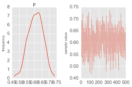
In [6]:
fit.plot('p');
plt.tight_layout()
Estimating mean and standard deviation of normal distribution
In [7]:
norm_code = """
data {
    int<lower=0> n;
    real y[n];
}
transformed data {}
parameters {
    real<lower=0, upper=100> mu;
    real<lower=0, upper=10> sigma;
}
transformed parameters {}
model {
    y ~ normal(mu, sigma);
}
generated quantities {}
"""

norm_dat = {
             'n': 100,
             'y': np.random.normal(10, 2, 100),
            }

fit = pystan.stan(model_code=norm_code, data=norm_dat, iter=1000, chains=1)
In [8]:
fit
Out[8]:
Inference for Stan model: anon_model_3318343d5265d1b4ebc1e443f0228954.
1 chains, each with iter=1000; warmup=500; thin=1;
post-warmup draws per chain=500, total post-warmup draws=500.

        mean se_mean     sd   2.5%    25%    50%    75%  97.5%  n_eff   Rhat
mu     10.07    0.02   0.22   9.64   9.91  10.07  10.22  10.48    133    1.0
sigma   2.02    0.01   0.15   1.76   1.93   2.01   2.12   2.33    127   1.02
lp__  -117.3     0.1   1.02 -119.9 -117.7 -117.0 -116.5 -116.2    103    1.0

Samples were drawn using NUTS(diag_e) at Tue Mar  1 07:31:19 2016.
For each parameter, n_eff is a crude measure of effective sample size,
and Rhat is the potential scale reduction factor on split chains (at
convergence, Rhat=1).
In [9]:
trace = fit.extract()
In [10]:
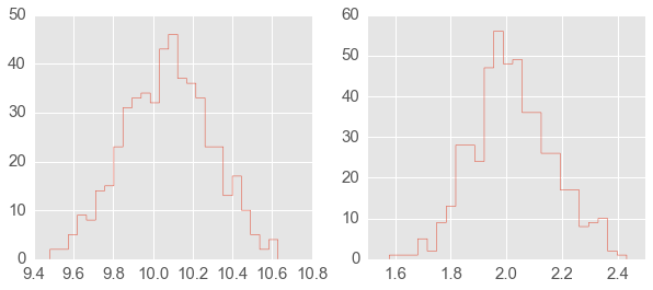
plt.figure(figsize=(10,4))
plt.subplot(1,2,1);
plt.hist(trace['mu'][:], 25, histtype='step');
plt.subplot(1,2,2);
plt.hist(trace['sigma'][:], 25, histtype='step');
Optimization (finding MAP)
In [11]:
sm = pystan.StanModel(model_code=norm_code)
op = sm.optimizing(data=norm_dat)
op
Out[11]:
OrderedDict([('mu', array(10.070206723560238)),
             ('sigma', array(1.9913542540072449))])
Reusing fitted objects
In [12]:
new_dat = {
             'n': 100,
             'y': np.random.normal(10, 2, 100),
            }
In [13]:
fit2 = pystan.stan(fit=fit, data=new_dat, chains=1)
In [14]:
fit2
Out[14]:
Inference for Stan model: anon_model_3318343d5265d1b4ebc1e443f0228954.
1 chains, each with iter=2000; warmup=1000; thin=1;
post-warmup draws per chain=1000, total post-warmup draws=1000.

        mean se_mean     sd   2.5%    25%    50%    75%  97.5%  n_eff   Rhat
mu      9.89    0.01    0.2   9.51   9.76   9.89  10.02  10.29    276    1.0
sigma    2.0  9.3e-3   0.14   1.75   1.89   1.99   2.08    2.3    226    1.0
lp__  -115.4    0.08   0.96 -118.2 -115.7 -115.1 -114.7 -114.5    151   1.01

Samples were drawn using NUTS(diag_e) at Tue Mar  1 07:32:02 2016.
For each parameter, n_eff is a crude measure of effective sample size,
and Rhat is the potential scale reduction factor on split chains (at
convergence, Rhat=1).
Saving compiled models
We can also compile Stan models and save them to file, so as to reload them for later use without needing to recompile.
In [17]:
def save(obj, filename):
    """Save compiled models for reuse."""
    import pickle
    with open(filename, 'wb') as f:
        pickle.dump(obj, f, protocol=pickle.HIGHEST_PROTOCOL)

def load(filename):
    """Reload compiled models for reuse."""
    import pickle
    return pickle.load(open(filename, 'rb'))
In [18]:
model = pystan.StanModel(model_code=norm_code)
save(model, 'norm_model.pic')
In [19]:
new_model = load('norm_model.pic')
fit4 = new_model.sampling(new_dat, chains=1)
fit4
Out[19]:
Inference for Stan model: anon_model_3318343d5265d1b4ebc1e443f0228954.
1 chains, each with iter=2000; warmup=1000; thin=1;
post-warmup draws per chain=1000, total post-warmup draws=1000.

        mean se_mean     sd   2.5%    25%    50%    75%  97.5%  n_eff   Rhat
mu       9.9    0.01    0.2   9.52   9.77    9.9  10.05  10.27    258    1.0
sigma   1.99  9.7e-3   0.15   1.73   1.89   1.98   2.08   2.32    252    1.0
lp__  -115.5    0.08   1.08 -118.5 -116.0 -115.2 -114.8 -114.5    167    1.0

Samples were drawn using NUTS(diag_e) at Tue Mar  1 07:48:40 2016.
For each parameter, n_eff is a crude measure of effective sample size,
and Rhat is the potential scale reduction factor on split chains (at
convergence, Rhat=1).
Estimating parameters of a linear regression model
We will show how to estimate regression parameters using a simple linear model
We can restate the linear model
as sampling from a probability distribution
We will assume the following priors
In [20]:
lin_reg_code = """
data {
    int<lower=0> n;
    real x[n];
    real y[n];
}
transformed data {}
parameters {
    real a;
    real b;
    real sigma;
}
transformed parameters {
    real mu[n];
    for (i in 1:n) {
        mu[i] <- a*x[i] + b;
        }
}
model {
    sigma ~ uniform(0, 20);
    y ~ normal(mu, sigma);
}
generated quantities {}
"""

n = 11
_a = 6
_b = 2
x = np.linspace(0, 1, n)
y = _a*x + _b + np.random.randn(n)

lin_reg_dat = {
             'n': n,
             'x': x,
             'y': y
            }

fit = pystan.stan(model_code=lin_reg_code, data=lin_reg_dat, iter=1000, chains=1)
In [21]:
fit
Out[21]:
Inference for Stan model: anon_model_4bdbb0aeaf5fafee91f7aa8b257093f2.
1 chains, each with iter=1000; warmup=500; thin=1;
post-warmup draws per chain=500, total post-warmup draws=500.

         mean se_mean     sd   2.5%    25%    50%    75%  97.5%  n_eff   Rhat
a        7.26     0.1   0.89   5.62   6.73   7.27   7.78   9.04     82   1.03
b        1.52    0.06   0.54   0.44    1.2   1.56   1.85   2.51     92   1.03
sigma    0.88    0.03   0.28   0.54    0.7   0.82   0.99   1.58     71   1.01
mu[0]    1.52    0.06   0.54   0.44    1.2   1.56   1.85   2.51     92   1.03
mu[1]    2.25    0.05   0.46   1.27   1.97   2.29   2.53   3.13     95   1.02
mu[2]    2.97    0.04   0.39   2.13   2.74   3.01    3.2   3.71    100   1.02
mu[3]     3.7    0.03   0.33   2.97   3.51   3.72   3.89   4.36    110   1.02
mu[4]    4.42    0.03   0.29   3.82   4.26   4.44    4.6   4.99    125   1.01
mu[5]    5.15    0.02   0.27   4.63   4.99   5.16   5.32   5.68    145    1.0
mu[6]    5.88    0.02   0.28    5.3   5.72   5.89   6.07   6.43    148    1.0
mu[7]     6.6    0.03   0.31   5.93   6.42   6.62   6.81   7.23    125    1.0
mu[8]    7.33    0.04   0.37   6.54   7.11   7.36   7.58   8.04    108   1.01
mu[9]    8.06    0.04   0.43   7.11    7.8   8.07   8.33   8.91     98   1.01
mu[10]   8.78    0.05   0.51   7.67   8.49   8.78   9.13   9.75     92   1.01
lp__    -3.27    0.23    1.7  -7.43  -3.94  -2.79  -2.04   -1.5     57    1.0

Samples were drawn using NUTS(diag_e) at Tue Mar  1 08:00:48 2016.
For each parameter, n_eff is a crude measure of effective sample size,
and Rhat is the potential scale reduction factor on split chains (at
convergence, Rhat=1).
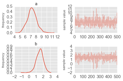
In [22]:
fit.plot(['a', 'b']);
plt.tight_layout()
Simple Logistic model
We have observations of height and weight and want to use a logistic model to guess the sex.
In [23]:
# observed data
df = pd.read_csv('HtWt.csv')
df.head()
Out[23]:
| male | height | weight | |
|---|---|---|---|
| 0 | 0 | 63.2 | 168.7 |
| 1 | 0 | 68.7 | 169.8 |
| 2 | 0 | 64.8 | 176.6 |
| 3 | 0 | 67.9 | 246.8 |
| 4 | 1 | 68.9 | 151.6 |
In [24]:
log_reg_code = """
data {
    int<lower=0> n;
    int male[n];
    real weight[n];
    real height[n];
}
transformed data {}
parameters {
    real a;
    real b;
    real c;
}
transformed parameters {}
model {
    a ~ normal(0, 10);
    b ~ normal(0, 10);
    c ~ normal(0, 10);
    for(i in 1:n) {
        male[i] ~ bernoulli(inv_logit(a*weight[i] + b*height[i] + c));
  }
}
generated quantities {}
"""

log_reg_dat = {
             'n': len(df),
             'male': df.male,
             'height': df.height,
             'weight': df.weight
            }

fit = pystan.stan(model_code=log_reg_code, data=log_reg_dat, iter=2000, chains=1)
In [25]:
fit
Out[25]:
Inference for Stan model: anon_model_bbf283522d1e199c049bb423b4a6e0da.
1 chains, each with iter=2000; warmup=1000; thin=1;
post-warmup draws per chain=1000, total post-warmup draws=1000.

       mean se_mean     sd   2.5%    25%    50%    75%  97.5%  n_eff   Rhat
a      0.25    0.11   0.19-4.4e-4   0.02   0.38    0.4   0.41      3   2.28
b     -0.61    0.28   0.48  -1.05  -1.01  -0.94  -0.01   0.03      3   2.34
c     -0.31    0.64   1.11   -2.3  -1.63   0.49    0.5    0.5      3   1.78
lp__ -191.2   66.47 115.13 -305.7 -289.3 -265.0 -47.06  -45.1      3   2.47

Samples were drawn using NUTS(diag_e) at Tue Mar  1 08:01:40 2016.
For each parameter, n_eff is a crude measure of effective sample size,
and Rhat is the potential scale reduction factor on split chains (at
convergence, Rhat=1).
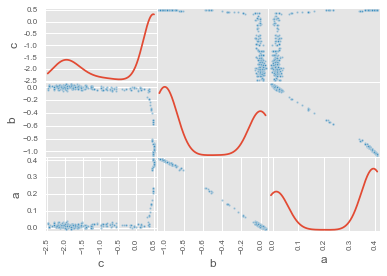
In [26]:
df_trace = pd.DataFrame(fit.extract(['c', 'b', 'a']))
pd.scatter_matrix(df_trace[:], diagonal='kde');
Estimating parameters of a logistic model
Gelman’s book has an example where the dose of a drug may be affected to the number of rat deaths in an experiment.
| Dose (log g/ml) | # Rats | # Deaths |
|---|---|---|
| -0.896 | 5 | 0 |
| -0.296 | 5 | 1 |
| -0.053 | 5 | 3 |
| 0.727 | 5 | 5 |
We will model the number of deaths as a random sample from a binomial distribution, where \(n\) is the number of rats and \(p\) the probability of a rat dying. We are given \(n = 5\), but we believe that \(p\) may be related to the drug dose \(x\). As \(x\) increases the number of rats dying seems to increase, and since \(p\) is a probability, we use the following model:
where we set vague priors for \(\alpha\) and \(\beta\), the parameters for the logistic model.
Original PyMC3 code
n = 5 * np.ones(4)
x = np.array([-0.896, -0.296, -0.053, 0.727])
y = np.array([0, 1, 3, 5])

def invlogit(x):
    return pm.exp(x) / (1 + pm.exp(x))

with pm.Model() as model:
    # define priors
    alpha = pm.Normal('alpha', mu=0, sd=5)
    beta = pm.Flat('beta')

    # define likelihood
    p = invlogit(alpha + beta*x)
    y_obs = pm.Binomial('y_obs', n=n, p=p, observed=y)

    # inference
    start = pm.find_MAP()
    step = pm.NUTS()
    trace = pm.sample(niter, step, start, random_seed=123, progressbar=True)
Exercise - convert to PyStan version
Using a hierarchical model
This uses the Gelman radon data set and is based off this IPython notebook. Radon levels were measured in houses from all counties in several states. Here we want to know if the preence of a basement affects the level of radon, and if this is affected by which county the house is located in.
The data set provided is just for the state of Minnesota, which has 85
counties with 2 to 116 measurements per county. We only need 3 columns
for this example county, log_radon, floor, where floor=0
indicates that there is a basement.
We will perform simple linear regression on log_radon as a function of county and floor.
In [ ]:
radon = pd.read_csv('radon.csv')[['county', 'floor', 'log_radon']]
radon.head()
Hiearchical model
With a hierarchical model, there is an \(a_c\) and a \(b_c\) for each county \(c\) just as in the individual county model, but they are no longer independent but assumed to come from a common group distribution
we further assume that the hyperparameters come from the following distributions
Original PyMC3 code
county = pd.Categorical(radon['county']).codes

with pm.Model() as hm:
    # County hyperpriors
    mu_a = pm.Normal('mu_a', mu=0, tau=1.0/100**2)
    sigma_a = pm.Uniform('sigma_a', lower=0, upper=100)
    mu_b = pm.Normal('mu_b', mu=0, tau=1.0/100**2)
    sigma_b = pm.Uniform('sigma_b', lower=0, upper=100)

    # County slopes and intercepts
    a = pm.Normal('slope', mu=mu_a, sd=sigma_a, shape=len(set(county)))
    b = pm.Normal('intercept', mu=mu_b, tau=1.0/sigma_b**2, shape=len(set(county)))

    # Houseehold errors
    sigma = pm.Gamma("sigma", alpha=10, beta=1)

    # Model prediction of radon level
    mu = a[county] + b[county] * radon.floor.values

    # Data likelihood
    y = pm.Normal('y', mu=mu, sd=sigma, observed=radon.log_radon)
Exercise - convert to PyStan version
In [ ]: