
Latest Revision: May 16, 1996
One can think of the buyer of the option paying a premium (price) for the option to buy a specified quantity at a specified price any time prior to the maturity of the option. Consider an example. Suppose you buy an option to buy 1 Treasury bond (coupon is 8%, maturity is 20 years) at a price of $76. The option can be exercised at any time between now and September 19th. The cost of the call is assumed to be $1.50. Let's tabulate the payoffs at expiration.
| Call Option Payoff | ||
|---|---|---|
| T-bond Price on Sept. 19 |
Gross Payoff on Option |
Net Payoff on Option |
| 60 | 0.0 | -1.5 |
| 70 | 0.0 | -1.5 |
| 75 | 0.0 | -1.5 |
| 76 | 0.0 | -1.5 |
| 77 | 1.0 | -0.5 |
| 78 | 2.0 | 0.5 |
| 79 | 3.0 | 1.5 |
| 80 | 4.0 | 2.5 |
| 90 | 14.0 | 12.5 |
| 100 | 24.0 | 22.5 |
Consider the payoffs diagrammatically. Notice that the payoffs are one to one after the price of the underlying security rises above the exercise price. When the security price is less than the exercice price, the option is referred to as out of the money.
A put option is a contact giving its owner the right to sell a fixed amount of a specified underlying asset at a fixed price at any time on or before a fixed date. On the expiration date, the value of the put on a per share basis will be the larger of the exercise price minus the stock price or zero.
One can think of the buyer of the put option as paying a premium (price) for the option to sell a specified quantity at a specified price any time prior to the maturity of the option. Consider an example of a put on the same Treasury bond. The exercise price is $76. You can exercise the option any time between now and September 19. Suppose that the cost of the put is $2.00.
| Put Option Payoff | ||
|---|---|---|
| T-bond Price on Sept. 19 |
Gross Payoff on Option |
Net Payoff on Option |
| 60 | 16.0 | 14.0 |
| 70 | 6.0 | 4.0 |
| 75 | 1.0 | -1.0 |
| 76 | 0.0 | -2.0 |
| 77 | 0.0 | -2.0 |
| 78 | 0.0 | -2.0 |
| 79 | 0.0 | -2.0 |
| 80 | 0.0 | -2.0 |
| 90 | 0.0 | -2.0 |
| 100 | 0.0 | -2.0 |
The payoff from a put can be illustrated. Notice that the payoffs are one to one when the price of the security is less than the exercise price.

Writing or "shorting" options have the exact opposite payoffs as purchased options. The payoff table for the call option is:
| Short Call Option Payoff | ||
|---|---|---|
| T-bond Price on Sept. 19 |
Gross Payoff on Option |
Net Payoff on Option |
| 60 | 0.0 | 1.5 |
| 70 | 0.0 | 1.5 |
| 75 | 0.0 | 1.5 |
| 76 | 0.0 | 1.5 |
| 77 | -1.0 | 0.5 |
| 78 | -2.0 | -0.5 |
| 79 | -3.0 | -1.5 |
| 80 | -4.0 | -2.5 |
| 90 | -14.0 | -12.5 |
| 100 | -24.0 | -22.5 |
Notice that the liability is potentially unlimited when you are writing options.

The put option can be similarly illustrated:
| Short Put Option Payoff | ||
|---|---|---|
| T-bond Price on Sept. 19 |
Gross Payoff on Option |
Net Payoff on Option |
| 60 | -16.0 | -14.0 |
| 70 | -6.0 | -4.0 |
| 75 | -1.0 | 1.0 |
| 76 | 0.0 | 2.0 |
| 77 | 0.0 | 2.0 |
| 78 | 0.0 | 2.0 |
| 79 | 0.0 | 2.0 |
| 80 | 0.0 | 2.0 |
| 90 | 0.0 | 2.0 |
| 100 | 0.0 | 2.0 |

As with the written call, the upside is limited to the premium of the option (the initial price). The downside is limited to the minimum asset price - which is zero.
There are two other definitions that are needed. A European Option is an option that can only be exercised at maturity. That is, there is no opportunity for early exercise. An American Option can be exercised at any time up to the maturity date.
Index Options
Index Option LEAPS (Long-term)
Oil Futures Options
Livestock Futures Options
Metals Futures Options
Interest Rate Futures Options
Currency Futures Options
Index Futures Options
Other Futures Options
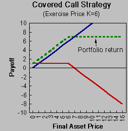
We can sketch the payoffs for this strategy. First, we need a few definitions. Let S^* be the ultimate value of the stock price on the maturity date. Let k be the exercise price. The call price will be denoted by c. The price of a zero coupon bond that matures on the same day as the option is denoted by B. The straight line is the payoffs from holding the stock long. The kinked solid line is the payoffs from shorting (writing) the call option. The dashed line is the net payoff. This is referred to as a hedge position. Note if the stock price stays below the exercise price, then you are clearly better off. If the stock price rises dramatically, then you do not capitalize on all the gain. The region below the dashed line denotes the gain from writing the covered call.
Suppose you have a choice of two investment strategies. The first is to invest $100 in a stock. The second strategy involves investing $90 in 6 month T-bills and $10 in 6 month calls. So we will want to buy 10/c calls. That is, if the call is priced at $5, then you are able to buy 2 calls.
The payoffs for this strategy are outlined below. Note that because we own 2 calls, the payoffs are two for one. That is for every dollar the stock price is above the exercise price, we make two dollars on the call. The diagram shows the payoffs from strategy 2. The slope of the call payoff is 2. The T-bill payout is flat. As soon as the stock price goes past the exercise price, the portfolio value rises rapidly. A comparison of the two investment strategies is outlined. Note that the option substitution strategy does not do as well if the stock price does not move that much.


As the current stock price goes up, the higher the probability that the call will be in the money. As a result, the call price will increase. The effect will be in the opposite direction for a put. As the stock price goes up, there is a lower probability that the put will be in the money. So the put price will decrease.
The higher the exercise price, the lower the probability that the call will be in the money. So for call options that have the same maturity, the call with the price that is closest (and greater than) the current price will have the highest value. The call prices will decrease as the exercise prices increase. For the put, the effect runs in the opposite direction. A higher exercise price means that there is higher probability that the put will be in the money. So the put price increases as the exercise price increases.
Both the call and put will increase in price as the underlying asset becomes more volatile. The buyer of the option receives full benefit of favorable outcomes but avoids the unfavorable ones (option price value has zero value).
The higher the interest rate, the lower the present value of the exercise price. As a result, the value of the call will increase. The opposite is true for puts. The decrease in the present value of the exercise price will adversely affect the price of the put option.
On ex-dividend dates, the stock price will fall by the amount of the dividend. So the higher the dividends, the lower the value of a call relative to the stock. This effect will work in the opposite direction for puts. As more dividends are paid out, the stock price will jump down on the ex-date which is exactly what you are looking for with a put. (There is also an issue of optimal exercise of the call and put option which will be addressed later.)
There are a number of effects involved here. Generally, both calls and puts will benefit from increased time to expiration. The reason is that there is more time for a big move in the stock price. But there are some effects that work in the opposite direction. As the time to expiration increase, the present value of the exercise price decreases. This will increase the value of the call and decrease the value of the put. Also, as the time to expiration increase, there is a greater amount of time for the stock price to be reduced by a cash dividend. This reduces the call value but increases the put value.
Let's summarize these effects.
| Effect of Increase on | |||
|---|---|---|---|
| |
|
Call Option |
Put Option |
| 1. | Current Stock Price | Increase | Decrease |
| 2. | Exercise Price | Decrease | Increase |
| 3. | Volatility | Increase | Increase |
| 4. | Interest Rates | Increase | Decrease |
| 5. | Dividends | Decrease | Increase |
| 6. | Time to Expiration | Increase | Increase |
Consider the following two rules:
(1) If one portfolio of securities gives a higher future payoff than another portfolio in every possible circumstance, then the first portfolio must have a higher current value than the second portfolio.
(2) If two portfolios of securities give the same future payoff in every possible circumstance, then they must have the same current value.
If (1) and (2) did not hold, then it would be possible for a professional trader to make an arbitrage profit by simultaneously selling the relatively overpriced portfolio and buying the relatively underpriced portfolio. We will use these rules to construct positions that offer the identical payoff as the option. If we can price the position with the same payoff as the option, then we have the price of the option.
Another point to note is that the modern valuation of exchange-traded options ignores margin requirements, transactions costs, and taxes because it focuses on market pricing relations that are enforced by the arbitrage activities of professional traders. The margin requirements and transactions costs of these traders are very low. Furthermore, taxes usually reduce the level of arbitrage profits but do not change the circumstances in which they occur.
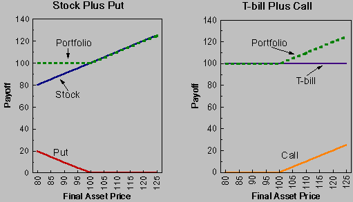
The price of a call and a put are linked via the put--call parity relationship. The idea here is that holding the stock and buying a put is going to deliver the exact same payoffs as buying one call and investing the present value of the exercise price. Let's demonstrate this. Consider the payoffs of two portfolios. Portfolio A contains the stock and a put. Portfolio B contains a call and an investment of the present value of the exercise price.
| Value on the Expiration Date | ||
|---|---|---|
| Action Today | S*<=k | S*>k |
| Buy one share | S* | S* |
| Buy one put | k- S* | 0 |
| Total | k | S* |
| Value on the Expiration Date | ||
|---|---|---|
| Action Today | S*<=k | S*>k |
| Buy one call | 0 | S*-k |
| Invest of PV of k | k | k |
| Total | k | S* |
Since the portfolios always have the same final value, they must have the same current value. This is the rule of no arbitrage. We can express the put--call parity relation as:
S+P=C+PV(k)
Of course, this relation can be written in many different ways:
P=C+PV(k) -S
C=S+P-PV(k)
and
C-P=S-PV(k)
where PV(k) is the present value of the exercise price. Now consider a diagram for each of the payoffs.
See also Option arbitrage relations.
We can also use the put-call parity theory for a stock that pays dividends. The idea is very similar to the no dividend case. The value of the call will be exactly equal to the value of a portfolio that includes the stock, a put, and borrowing the present value of the dividend and the present value of the exercise price. Consider the payoffs of two portfolios. Portfolio A just contains the call option. Portfolio B contains the stock, a put and borrowing equal to the present value of the exercise price and the present value of the dividend.
| Value on the Expiration Date | ||
|---|---|---|
| Action Today | S*<=k | S*>k |
| Buy one call | 0 | S*-k |
| Total | 0 | S*-k |
| Value on the Expiration Date | ||
|---|---|---|
| Action Today | S*<=k | S*>k |
| Buy one share | S* | S* |
| Buy one put | k- S* | 0 |
| Borrow the PV of k and d | -k | -k |
| Total | 0 | S*-k |
Since the portfolios always have the same final value, they must have the same current value. Again, this is the rule of no arbitrage. Note that this arrangement of the portfolios is slightly different from the case with no dividends. In the no dividends case, we had the stock and a put in portfolio A. In the dividends case, we have just the call in portfolio A. But clearly, we could have constructed the no dividends case with just a call in the portfolio A -- it would have no impact on the result. Further note, that the as result of borrowing the present value of both the dividend and the exercise price, we only payoff the exercise price. The reason for this is that if you get the dividend payment before expiration, then you use it to reduce you total debt. In fact, you use it to exactly payoff that part of the debt that is related to the dividend part of the borrowing.
We can express the put--call parity relation as:
c=S +p -PV(k)-PV(d)
where PV(k) is the present value of the exercise price and PV(d) is the present value of the dividend. We can be more precise about these present values:

Note that we are using continuous time rates of interest here. All that is really happening is that you are selling k zero coupon bonds today. At the time of expiration, T, you have to pay those bonds off. The amount that you have to payoff is k. You are also selling d zero coupons bonds which mature at the date that the dividend is paid, T_1. For these bonds, you use the revenue from the dividend paid to pay off the bonds.
Consider the time line:

S+P=C+PV(k)
Xerox stock sells for $61. The Xerox/April/60 call sells for $7 3/8 and the Xerox/April/60 put sells for $3 1/4. The call, put and a Treasury Bill all mature in 4 months. The Treasury Bill price is .9492. Assume that Xerox does not pay dividends in this period. Draw the position diagram for (a) long one call, (b) short one call, long one share of the stock (c) long one put. Using the call, put, stock and bond, demonstrate how you can make arbitrage profits. Ignore dividends, premature exercise, and transactions costs.
(a)

(b)

(c)

First, note that all the position diagrams are drawn at the time of expiration. Second, these diagrams are net positions. [Aside: Note that is possible to put the cost of the call or the put terms of time T dollars. We know the price of the Treasury bill is .9492 so we can calculate the future values of original call price and put price. c=7+ 3/8=7.375; c/B=7.77 and p=3 1/4=3.25; p/B=3.42. However, the convention is to present the payoff tables and diagrams in terms of the time at expiration.]
Now consider the possibility of arbitrage profits today. We can use the put-call parity relation.
c-p-S+PV(k)=0
We know the value of all of these variables. The present value of the exercise price is:
60 x .9492=56.95
So just plug into the put-call parity relation:
7.38-3.25-61+56.95=0.08
This inflow is very close to zero and will be wiped out by transactions costs and the bid-ask spread. The put-call parity condition is satisfied well.
Once again, consider two portfolios A and B.
| Value on the Expiration Date | ||
|---|---|---|
| Action Today | S*<=k | S*>k |
| Buy one call | 0 | S*-k |
| Total | 0 | S*-k |
| Value on the Expiration Date | ||
|---|---|---|
| Action Today | S*<=k | S*>k |
| Buy one share | S* | S* |
| Borrow PV of k | -k * | -k |
| Total | S* -k | S* -k |
So the value of portfolio A>=q the value of portfolio B. Which means that the current call value is greater than or equal to the current stock price less the present value of the exercise price. Note that the only difference between these portfolios and the portfolios we used for put-call parity is the absence of the put option. Note also that dividends are not included in this example. If the stock is paying dividends, this minimum value will no longer be appropriate. The terminal value of portfolio B would include the accumulated dividends, so the call would no longer always have a larger payoff. To adjust for the dividend, we could change the composition of portfolio B. Instead of simply buying and holding one share, as we did with no dividends, we would now want a strategy that would:
The exact form of the strategy would depend upon the dividend strategy of the firm. The minimum value of the call with a stock that pays dividends can be represented in the following table.
| Value on the Expiration Date | ||
|---|---|---|
| Action Today | S*<=k | S*>k |
| Buy one call | 0 | S*-k |
| Total | 0 | S*-k |
| Value on the Expiration Date | ||
|---|---|---|
| Action Today | S*<=k | S*>k |
| Buy one share | S* | S* |
| Borrow PV of k and d | -k * | -k |
| Total | S* -k | S* -k |
In this case, the value of portfolio A>=q the value of portfolio B. This means that the current call value is greater than or equal to the current stock price less the present value of the exercise price and the present value of the dividend payment. The idea here is that you use the dividends received from the stock to pay off the loan of the present value of the dividends. Note that the only difference between these portfolios and the portfolios we used for put-call parity is the absence of the put option.
The maximum value of a call option is easier to determine than the minimum value. Simply stated, the value of the call option can never exceed the stock price. This is true because we can consider the stock itself as a call option. The exercise price of the option is $0 and the time to maturity is infinite.
We know that the lower the exercise price, the higher the value of the call. This is because there is a higher probability that the call will be in the money. With the stock, the exercise price is zero. The exercise prices for traded options are never zero. This implies that the call will not be worth more than the stock.
We also know that a longer time to maturity will increase the value of the call (and put). This is because there is more time for a big move in the stock price. The stock is an option with infinite maturity. So it makes sense that the call should never be worth more than the stock.

The implication here is that if the stock price is zero the call will also be worth zero. The we can show the boundaries of the call price diagrammatically.

The upper bound in this diagram is the call price equalling the stock price. The lower bound is the call price equaling the stock price minus the present value of the exercise price (no dividends case). Since we know that the price of the call is zero if the stock price is zero, we know at least one point on the graph. The dashed line represents the call price today. Note that the price always stays within the boundaries. Note further that the call is convex in the stock price. Convexity means that if you draw a straight line between any two points on the call curve, all of the values in between these points are below the straight line.
We conjectured that the call and the put would increase in value if the expected volatility of the underlying asset increased. The intuition was that the greater the volatility the greater the chance for a big move -- either up or down. Both the call and the put would benefit from the greater probability of a big move. The following is a proof by example of this property. Suppose we have an XXX call option. The exercise price is $70 and the current XXX price is $66.75.
| Today's price |
Possible prices |
Call payoff |
Low volatility probability |
High volatility probability |
|---|---|---|---|---|
| 60 | 0 | .10 | .15 | |
| 65 | 0 | .20 | .25 | |
| 66.75 | 70 | 0 | .35 | .25 |
| 75 | 5 | .25 | .25 | |
| 80 | 10 | .10 | .15 | |
| 1.0 | 1.0 |
The expected call payoff for the low variance scenario is $2.25 and the expected call payoff for the high variance scenario is $2.75. This proves that a higher variance of the asset's expected price implies a higher expected payoff on the option. This implies that option buyers like high variance for its effect on the expected option payoff -- not because investors like variance.
The normal distribution is a continuous bell--shaped probability distribution. The normal distribution is particularly convenient to use because the distribution can be completely described by two parameters -- the mean and the variance. Below is a diagram of a normal distribution and the actual U.S. stock returns. That is, this distribution is drawn with the historical mean and variance of the U.S. stock returns.

We will work with the "standard" normal. This distribution is called standard because the mean is assumed to be zero and the standard deviation is one. The area under the normal curve represents the probability. In all the options pricing examples we will be interested in cumulative probability. The interpretation is: what is the probability that the value is less than some number, x. This simply means that we are going to be summing up the area under the curve -- working from the left.
Let's consider an example. If I am given the number zero, what is the cumulative probability. Stated differently, what is the probability that the number that I draw from the distribution has the value of negative infinity to zero. What I want is the area under the curve to the left of zero. Since the curve is symmetric and since the area under the curve must sum to one, the probability is .50. If I am given the number -3, what is the probability? Viewing the diagram of the normal distribution, the -3 is way out on the left tail. The area from -3 to the left is very small (a guess would be .01). If we were given the point 3, this is way out on the right tail. The area to the left of 3 is almost the entire area under the curve (a guess would be .99).
In order to use the Black-Scholes formula, we need precise numbers for these probabilities. We usually use a computer or a statistical table to get these probabilities.
We will denote the cumulative normal by N(x)=prob. Some examples are
 N(x=0)			=.50
 N(x=1)			=.8413
 N(x=-1)=1-N(1) 	=.1587
 N(x=1.96)		=.975
 N(x=-1.96)=1-N(1.96)	=.025
The formula for the normal distribution is:

First, some definitions are needed.
The Black-Scholes Formula:

There are many ways of writing the Black-Scholes formula. All of them are equivalent to the above. For example, Sharpe's text presents the formula differently. However, with some algebra, the formula is identical to the Black and Scholes formula above.
Now to get used to using the formula, it is best to do some examples. I will show how to use Black Scholes tables to get the price of the call option. However, everyone should be able to code the formula into an EXCEL spreadsheet..
But before we work some examples, I will try to given some of the intuition behind the formula.
Usually, in Finance, we refer to people as risk averse. I defined this earlier as the preference for $50 for sure rather than taking a 50-50 bet with payoffs of $0 and $100. Now let's suppose that agents are risk neutral. This means that they are indifferent between the $50 for sure and the bet. If this is the case, then the value of the call can be thought of as the expected payoff of the call at expiration discounted back to present value. We could write:

Note that S^* is the stock price at expiration. This expression says that the call price is the present value of the expected expiration price minus the exercise price times the probability the call is in the money.
In terms of the Black-Scholes formula, N(x_2) can be interpreted as the probability that the call option will be in the money at expiration. The term N(x_1) is the present value of the expected terminal stock price conditional upon the call option being in the money at expiration times the probability that the call will be in the money at expiration. Finally, the term e^{-rT}kN(x_2) is the present value of the cost of exercising the option at expiration times the probability that the call will be in the money at expiration. So the Black-Scholes formula for call option has a fairly simple interpretation. The call price is simply the discounted expected value of the cash flows at expiration.
(b) Value a 5 month IBM call with the same terms.
(c) If the current prices of these two calls are $15.75 for the 5 month and $12.12 for the 2 month, then are these options overvalued or undervalued according to the Black-Scholes formula.
(d) What are the potential causes of these discrepancies?
(e) What standard deviation is implied by the current market price of the 5 month call option (approximately)?
(a) The information that we know is: S=265, k=260, T=2/12=.166, 'sigma'=.30, r=.07, dividend yield=.04. First, let's adjust the stock price for the dividend.

The 'delta' is .04 and we are assuming a continuous dividend payout. The 263.24 represents the stock price minus the present value of the dividend.
Next compute the present value of the exercise price.

Step One. Calculate the ex-dividend stock price divided by the present value of the exercise price.

Step Two. Calculate the standard deviation of the stock's return to maturity.

Step Three. Go to the option tables. Along the top of the table is find 1.02 and at the same time search for the row 0.123. Since the table does not have such a fine division, interpolate between 0.10 and 0.15. Black-Scholes Tables. The approximate value is 6.1%. This is represents the call option price as a percentage of the ex-dividend stock price. To get the value of the call option, multiply 6.1% by the adjusted stock price:
c=.061 x 263.23=$16.06
Since we are interpolating from a table this is only an approximation. It roughly matched the call price from our previous solution.
(b) Follow the same steps as (a). Now we are considering T=5/12.
Step One. Calculate the ex-dividend stock price divided by the present value of the exercise price.

Step Two. Calculate the standard deviation of the stock's return to maturity.

Step Three. Go to the tables. Along the top of the table is find 1.03 and at the same time search for the row 0.194. Since the table does not have such a fine division, interpolate between 1.02 and 1.03 along the top and use 0.20 along the side. Black-Scholes Tables. The approximate value is 9.3%. This is represents the call option price as a percentage of the ex-dividend stock price. To get the value of the call option, multiply 9.3% by the adjusted stock price:
c=.093 x 260.62=$24.23
Since we are interpolating from a table this is only an approximation. It almost exactly matches the call price from our previous solution ($24.31).
(c) According to these assumptions and the Black-Scholes formula, market is currently undervaluing these calls:
12.12<$16.06 2 month
and 15.75<$24.31 5 month
(d) The major sources for error are: (1) the Black-Scholes assumptions are incorrect or (2) the estimated 'sigma' is incorrect.
(e) This question asks us to calculate the 'sigma' that makes the Black-Scholes call price exactly equal to the market price. The sigma that we get will not equal the .30 that we were given. It will be called the implied standard deviation. It turns out that there is no direct way to solve for this implied measure. The implied standard deviation can be obtained using tables (which is the next approach). One can also use SOLVER in EXCEL to get the implied standard deviation.
Calculate the ratio of the actual call price to the ex-dividend stock price.

We know from before that ratio of the ex-dividend stock price to the present value of the exercise price was 1.024. From the table search for a 'sigma'\sqrt T that when matched with 1.024 delivers 4.6%. Black-Scholes Tables. That value turns out to be about .083. To get the annualized implied standard deviation divide by the square root of T.

We can compute the same quantity for the 5 month call. The ratio of the actual call price to the ex-dividend stock price is:

The ratio of the ex-dividend stock price to the present value of the exercise price is 1.032 from before. Black-Scholes Tables. The 'sigma'\sqrt T that approximately matches these two quantities is .11. So the annual standard deviation is

The option delta measures the change in the option price for a unit change in the stock price.
The delta is also known as the hedge ratio. This means that the delta tells how many shares I need to buy to hedge the sale of one call. We can calculate the delta of a call option the same way using the tables. Black-Scholes Tables.

Of course, we get more precise answers on the computer. Unfortunately, this year, we do not allow computers into the exam. However, this will change!
The precise formula for the delta is:

The elasticity or 'omega' is interpreted as the call option's elasticity to changes in the underlying asset's price. So if the stock price rises by 1% the call price should rise by 'omega'%. We can now see the link between the delta and the omega.

We can calculate the 'omega' of a call option the same way using the tables.
The delta of a call option is the first derivative of the Black-Scholes call formula with respect to the stock price:

The delta of a put option is the first derivative of the put formula with respect to the stock price. From put-call parity, we know.

The delta of the put is:

The omega of the call option is

Similarly, the omega of the put option is
