Principles and risks
of forecasting (pdf)
Famous forecasting
quotes
How to move data around
Get to know your data
Inflation adjustment (deflation)
Seasonal adjustment
Stationarity and differencing
The logarithm
transformation
Introduction to logarithms
Change in natural log ≈ percentage change
Linearization of exponential growth and inflation
Trend measured in natural-log units ≈ percentage growth
Errors measured in natural-log units ≈ percentage
errors
Coefficients in log-log regressions ≈ proportional percentage
changes
Introduction to logarithms: Logarithms are one of the most
important mathematical tools in the toolkit of statistical modeling, so you
need to be very familiar with their properties and uses. A
logarithm function is defined with respect to a “base”, which is a
positive number: if b denotes the base number, then the
base-b logarithm of X is, by definition, the number Y such that bY =
X. For example, the base-2
logarithm of 8 is equal to 3, because 23 = 8, and the base-10
logarithm of 100 is 2, because 102 = 100. There are three kinds of logarithms
in standard use: the base-2 logarithm (predominantly used in computer science
and music theory), the base-10 logarithm (predominantly used in engineering),
and the natural logarithm (predominantly used in mathematics and
physics and in economics and business). In the natural log function, the base
number is the transcendental number “e”
whose deciminal expansion is 2.718282…, so the natural log function and
the exponential function (ex)
are inverses of each other. The
only differences between these three logarithm functions are multiplicative
scaling factors, so logically they are equivalent for purposes of modeling, but
the choice of base is important for reasons of convenience and convention,
according to the setting.
In standard mathematical notation, and in Excel and most
other analytic software, the expression LN(X) is the natural log of X, and
EXP(X) is the exponential function of X, so EXP(LN(X)) = X and LN(EXP(X)) =
X. This means that the EXP function can be used to convert
natural-logged forecasts (and their respective lower and upper confidence
limits) back into real units.
You cannot use the EXP function to directly unlog the error statistics of a model fitted to
natural-logged data. You need to
first convert the forecasts back into real units and then recalculate the
errors and error statistics in real units, if it is important to have those
numbers. However, the error
statistics of a model fitted to natural-logged data can often be interpreted as
approximate measures of percentage
error, as explained below, and in situations where logging is appropriate in
the first place, it is often of interest to measure and compare errors in
percentage terms.
In general, the expression LOGb(.) is used to denote the base-b logarithm function,
and LN is used for the special case of the natural log while LOG is often used
for the special case of the base-10 log. In particular, LOG means base-10 log in
Excel. In Statgraphics, alas, the function that
is called LOG is the natural log,
while the base-10 logarithm function is LOG10. In the remainder of this section (and
elsewhere on the site), both LOG and LN will be used to refer to the natural log function, for compatibility with
Statgraphics notation. Also,
the symbol “≈”
means approximately equal, with the
approximation being more accurate in relative terms for smaller absolute
values, as shown in the table below.
Change in
natural log ≈ percentage change: The natural
logarithm and its base number e have some magical properties, which you
may remember from calculus (and which you may have hoped you would never meet
again). For example, the function eX is its own derivative,
and the derivative of LN(X) is 1/X. But for purposes of
business analysis, its great advantage is that small changes in the natural
log of a variable are directly interpretable as percentage changes,
to a very close approximation.
The reason for this is that the graph of Y = LN(X) passes
through the point (1, 0) and has a slope of 1 there, so it is tangent to the
straight line whose equation is Y = X-1 (the dashed line in the plot
below):
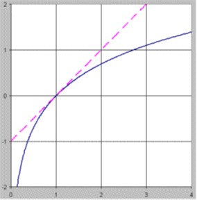
This
property of the natural log function implies that
LN(1+r) ≈ r
when
r is much smaller than 1 in magnitude.
Why is this important?
Suppose X increases by a small
percentage, such as 5%. This means
that it changes from X to X(1+r),
where r = 0.05. Now observe:
LN(X (1+r)) =
LN(X) + LN(1+r) ≈
LN(X) + r
Thus,
when X is increased by 5%, i.e., multiplied by a factor of 1.05, the natural
log of X changes from LN(X) to LN(X) + 0.05, to a very close
approximation. Increasing X by 5%
is therefore (almost) equivalent to adding 0.05 to LN(X).
From
now on I will refer to changes in natural logarithms as
“diff-logs.” (In
Statgraphics, the diff-log transformation of X is literally DIFF(LOG(X)).) The following table shows the exact
correspondence for percentages in the range from -50% to +100%:
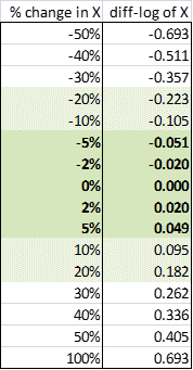
As you can see, percentage changes and
diff-logs are almost exactly the same within the range +/- 5%, and they remain
very close up to +/- 20%. For large
percentage changes they begin to diverge in an asymmetric way. Note that the diff-log that corresponds
to a 50% decrease is ‑0.693 while the diff-log of a 100% increase is
+0.693, exactly the opposite number.
This reflects the fact that a 50% decrease followed by a 100% increase
(or vice versa) takes you back to the same spot.
The
percentage change in Y at period t is defined as (Yt-Yt-1)/Yt-1,
which is only approximately equal to LN(Yt) - LN(Yt-1),
but the approximation is almost exact if the percentage change is small,
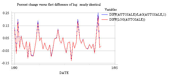
as shown in the table above. In
Statgraphics terms, this means that DIFF(Y)/LAG(Y,1) is virtually identical to
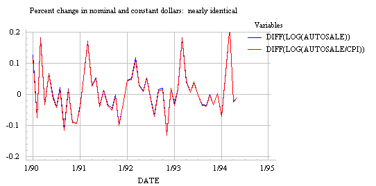
DIFF(LOG(Y)). If you don't believe
me, here's a plot of the percent change in auto sales versus the first
difference of its logarithm, zooming in on the last 5 years. The blue and
red lines are virtually indistinguishable except at the highest and lowest
points. (Again, LOG means LN in Statgraphics.)
If the situation
is one in which the percentage changes are potentially large enough for this
approximation to be inaccurate, it is better to use log units rather than
percentage units, because this takes compounding into account in a systematic
way, and it is symmetric in terms of sequences of gains and losses.
A diff-log of -0.5 followed by a diff-log of +0.5 takes you back to
your original position, whereas a 50% loss followed by a 50% gain (or vice
versa) leaves you in a worse position.
(Return to top of page.)
Linearization
of exponential growth and inflation:
The logarithm of a product equals the
sum of the logarithms, i.e., LOG(XY) = LOG(X) + LOG(Y), regardless of the
logarithm base. Therefore, logging converts multiplicative relationships
to additive relationships, and by the same token it converts exponential
(compound growth) trends to linear trends. By taking logarithms of variables which
are multiplicatively related and/or growing exponentially over time, we can
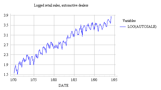
often explain their behavior with linear models. For example, here is a graph
of LOG(AUTOSALE). Notice that the
log transformation converts the
exponential growth pattern to a linear
growth pattern, and it simultaneously converts the multiplicative (proportional-variance) seasonal pattern to an additive (constant-variance) seasonal
pattern. (Compare this with the original graph of AUTOSALE.) These
conversions make the transformed data much more suitable for fitting with
linear/additive models.
Logging a series often has an effect very similar to deflating: it straightens
out exponential growth patterns and reduces heteroscedasticity (i.e., stabilizes
variance). Logging is therefore a "poor
man's deflator" which does not require any external data (or any
head-scratching about which price index to use). Logging is not exactly
the same as deflating--it does not eliminate an upward trend in the
data--but it can straighten the trend out so that it can be better fitted by a
linear model. Deflation by itself
will not straighten out an exponential growth curve if the growth is partly
real and only partly due to inflation.
If you're
going to log the data and then fit a model that implicitly or explicitly uses differencing
(e.g., a random walk, exponential smoothing, or ARIMA model), then it is
usually redundant to deflate by a price index, as long as the rate of inflation
changes only slowly: the percentage change measured in nominal dollars will be
nearly the same as the percentage change in constant dollars. In Statgraphics
notation, this means that, DIFF(LOG(Y/CPI)) is nearly identical to DIFF(LOG(Y)):
the only difference between the two is a very faint amount of noise due to fluctuations
in the inflation rate. To demonstrate this point, here's a graph of the first
difference of logged auto sales, with and without deflation:
By logging
rather than deflating, you avoid the need to incorporate an explicit
forecast of future inflation into the model: you merely lump inflation together
with any other sources of steady compound growth in the original data. Logging
the data before fitting a random walk model yields a so-called geometric random walk--i.e.,
a random walk with geometric rather than linear growth. A geometric random walk
is the default forecasting model that is commonly used for stock price data. (Return to top of page.)
Trend
measured in natural-log units ≈ percentage growth: Because changes in the natural logarithm are (almost) equal
to percentage changes in the original series, it follows that the slope
of a trend line fitted to logged data is equal to the average percentage
growth in the original series. For example, in the graph of LOG(AUTOSALE) shown above, if you "eyeball" a
trend line you will see that the magnitude of logged auto sales increases by
about 2.5 (from 1.5 to 4.0) over 25 years, which is an average increase of
about 0.1 per year, i.e., 10% per year. It is much easier to
estimate this trend from the logged graph than from the original unlogged
one! The 10% figure obtained here is nominal growth, including
inflation. If we had instead eyeballed a trend line on a plot of logged deflated
sales, i.e., LOG(AUTOSALE/CPI), its slope would be the average real percentage
growth.
Usually the trend is estimated more precisely by fitting a statistical model
that explicitly includes a local or global trend parameter, such as a linear
trend or random-walk-with-drift or linear exponential smoothing model.
When a model of this kind is fitted in conjunction with a log transformation,
its trend parameter can be interpreted as a percentage growth rate.
Errors
measured in natural-log units ≈ percentage errors: Another interesting property of the logarithm is that
errors in predicting the logged series can be interpreted as approximate
percentage errors in predicting the original series, albeit the percentages are
relative to the forecast values, not the actual values. (Normally one
interprets the "percentage error" to be the error expressed as a
percentage of the actual value, not the forecast value, although the
statistical properties of percentage errors are usually very similar regardless
of whether the percentages are calculated relative to actual values or
forecasts.)
Thus, if
you use least-squares estimation to fit a linear forecasting model to logged
data, you are implicitly minimizing mean squared percentage error,
rather than mean squared error in the original units, which is probably a good
thing if the log transformation was appropriate in the first place. And if you
look at the error statistics in logged units, you can interpret them as
percentages if they are not too large--say, if their standard deviation is 0.1
or less. Within this range, the
standard deviation of the errors in predicting a logged series is approximately
the standard deviation of the percentage errors in predicting the original
series, and the mean absolute error (MAE) in predicting a logged series is
approximately the mean absolute percentage error (MAPE) in predicting the
original series. (I am using a
benchmark of 0.1 here because at that point a 2 standard deviation variation,
the critical value for a 95% confidence interval, would be 0.2, and the
correspondence between diff-logs and percentages begins to fall off pretty
rapidly beyond that as shown in the table above. If the error standard deviation in
logged units is larger than 0.1, you ought to calculate confidence limits in
logged units and then un-log their lower and upper values separately by using
the EXP function.)
Coefficients
in log-log regressions ≈ proportional percentage changes: In many economic situations (particularly
price-demand relationships), the marginal effect of one variable on the
expected value of another is linear in terms of percentage changes rather than absolute
changes. In such cases, applying a
natural log or diff-log transformation to both dependent and independent
variables may be appropriate. This
issue will be discussed in more detail in the regression chapter of these
notes. In particular, part 3 of the beer sales
regression example illustrates an application of the log transformation in
modeling the effect of price on demand, including how to use the EXP
(exponential) function to “un-log” the forecasts and confidence limits
to convert them back into the units of the original data.
