 Averaging and smoothing models
Notes
on forecasting with moving averages (pdf)
Averaging and exponential
smoothing models
Slides
on inflation and seasonal adjustment and Winters seasonal exponential smoothing
Spreadsheet
implementation of seasonal adjustment and exponential smoothing
Equations
for the smoothing models (SAS web site)
Spreadsheet
implementation of seasonal adjustment and exponential smoothing
It is
straightforward to perform seasonal adjustment and fit exponential smoothing
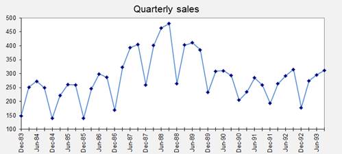
models using Excel. The screen images and charts below are taken from a
spreadsheet which has been set up to illustrate multiplicative seasonal
adjustment and linear exponential smoothing on the following quarterly sales
data from Outboard Marine:
To obtain
a copy of the spreadsheet file itself, click here. The version of linear exponential
smoothing that will be used here for purposes of demonstration is Brown’s
version, merely because it can be implemented with a single column of formulas
and there is only one smoothing constant to optimize. Usually it is better to use Holt’s
version that has separate smoothing constants for level and trend.
The
forecasting process proceeds as follows: (i) first the data are seasonally
adjusted; (ii) then forecasts are generated for the seasonally adjusted data
via linear exponential smoothing; and (iii) finally the seasonally adjusted
forecasts are "reseasonalized" to obtain forecasts for the original
series. The seasonal adjustment process is carried out in columns D through G.
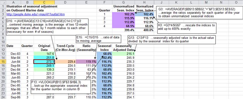
The first
step in seasonal adjustment is to compute a centered moving average
(performed here in column D). This can be done by taking the average of two
one-year-wide averages that are offset by one period relative to each other. (A
combination of two offset averages rather than a single average is needed for
centering purposes when the number of seasons is even.) The next step is to
compute the ratio to moving average--i.e., the original data divided by
the moving average in each period--which is performed here in column E. (This is also called the "trend-cycle"
component of the pattern, insofar as trend and business-cycle effects might be
considered to be all that remains after averaging over a whole year's worth of
data. Of course, month-to-month changes that are not due to seasonality could be
determined by many other factors, but the 12-month average smooths over them to
a great extent.) The
estimated seasonal index for each season is computed by first averaging
all the ratios for that particular season, which is done in cells G3-G6 using
an AVERAGEIF formula. The average
ratios are then rescaled so that they sum to exactly 100% times the number of
periods in a season, or 400% in this case, which is done in cells H3-H6.
Below in column F, VLOOKUP formulas are used to insert the appropriate seasonal
index value in each row of the data table, according to the quarter of the year
it represents. The centered
moving average and the seasonally adjusted data end up looking like this:

Note that
the moving average typically looks like a smoother version of the seasonally
adjusted series, and it is shorter on both ends.
Another
worksheet in the same Excel file shows the
application of the linear exponential smoothing model to the seasonally
adjusted data, beginning in column G.
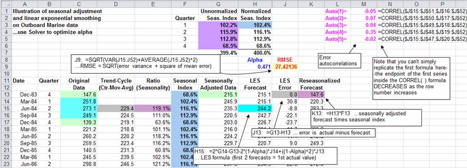
A value
for the smoothing constant (alpha) is entered above the forecast column (here,
in cell H9) and for convenience it is assigned the range name
"Alpha." (The name is assigned using the
"Insert/Name/Create" command.) The LES model is initialized by
setting the first two forecasts equal to the first actual value of the
seasonally adjusted series. The formula used here for the LES forecast is the
single-equation recursive form of Brown’s model:
![]()
This formula is entered in the cell corresponding to the third period (here,
cell H15) and copied down from there. Notice that the LES forecast for the
current period refers to the two preceding observations and the two
preceding forecast errors, as well as to the value of alpha. Thus, the
forecasting formula in row 15 refers only to data which were available in row
14 and earlier. (Of course, if we wished to use simple instead of linear
exponential smoothing, we could substitute the SES formula here instead. We could also use Holt’s rather
than Brown’s LES model, which would require two more columns of formulas
to calculate the level and trend that are used in the forecast.)
The errors
are computed in the next column (here, column J) by subtracting the forecasts
from the actual values. The root
mean squared error is computed as the square root of the variance of
the errors plus the square of the mean. (This follows from the mathematical
identity: MSE = VARIANCE(errors)+ (AVERAGE(errors))^2.) In calculating the mean
and variance of the errors in this formula, the first two periods are excluded
because the model does not actually begin forecasting until the third period
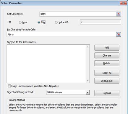
(row 15 on the spreadsheet). The optimal value of alpha can be found either by
manually changing alpha until the minimum RMSE is found, or else you can use
the "Solver" to perform an exact minimization. The value of alpha
that the Solver found is shown here (alpha=0.471).
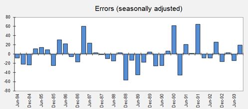
It is
usually a good idea to plot the errors of the model (in transformed units) and
also to compute and plot their autocorrelations at lags of up to one season.
Here is a time series plot of the (seasonally adjusted) errors:
The error
autocorrelations are computed by using the CORREL( ) function to compute the
correlations of the errors with themselves lagged by one or more periods--details
are shown in the spreadsheet model. Here is a plot of the autocorrelations of
the errors at the first five lags:
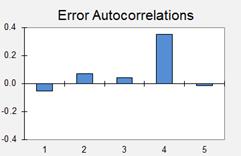
The
autocorrelations at lags 1 to 3 are very close to zero, but the spike at lag 4
(whose value is 0.35) is slightly troublesome--it suggests that the seasonal
adjustment process has not been completely successful. However, it is actually
only marginally significant. 95%
significance bands for testing whether autocorrelations are significantly
different from zero are roughly plus-or-minus 2/SQRT(n-k), where n is the sample size
and k is the lag. Here n is 38 and k varies from 1 to 5, so the
square-root-of-n-minus-k is around 6 for all of them, and hence the limits for
testing the statistical significance of deviations from zero are roughly
plus-or-minus 2/6, or 0.33. If you vary the value of alpha by hand in this
Excel model, you can observe the effect on the time series and autocorrelation
plots of the errors, as well as on the root-mean-squared error, which will be
illustrated below.
At the
bottom of the spreadsheet, the forecasting formula is "bootstrapped"
into the future by merely substituting forecasts for actual values at the point
where the actual data runs out--i.e., where "the future" begins. (In
other words, in each cell where a future data value would occur, a cell
reference is inserted which points to the forecast made for that
period.) All the other formulas are simply copied down from above:
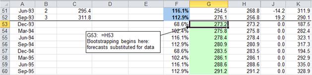
Notice that
the errors for forecasts of the future are all computed to be zero.
This does not mean the actual errors will be zero, but rather it merely
reflects the fact that for purposes of prediction we are assuming that the
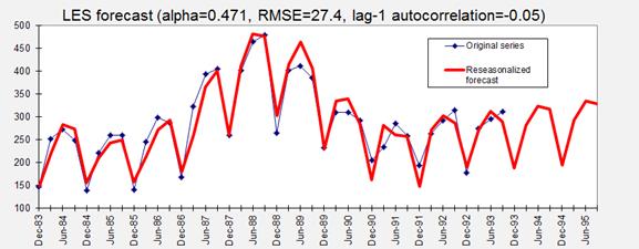
future data will equal the forecasts on average. The resulting LES
forecasts for the seasonally adjusted data look like this:
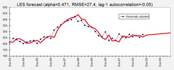
With this
particular value of alpha, which is optimal for one-period-ahead predictions,
the projected trend is slightly upward, reflecting the local trend that was
observed over the last 2 years or so. For other values of alpha, a very
different trend projection might be obtained. It is usually a good idea to see
what happens to the long-term trend projection when alpha is varied, because
the value that is best for short-term forecasting will not necessarily be the
best value for predicting the more distant future. For example, here is the
result that is obtained if the value of alpha is manually set to 0.25:
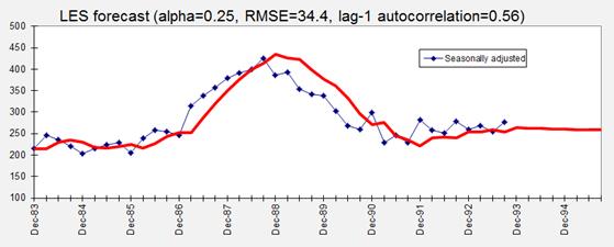
The
projected long-term trend is now negative rather than positive! With a smaller
value of alpha, the model is placing more weight on older data in its
estimation of the current level and trend, and its long-term forecasts reflect
the downward trend observed over the last 5 years rather than the more recent
upward trend. This chart also clearly illustrates how the model with a smaller
value of alpha is slower to respond to "turning points" in the data
and therefore tends to make an error of the same sign for many periods in a
row. Its 1-step-ahead forecast
errors are larger on average than those obtained before (RMSE of 34.4 rather
than 27.4) and strongly positively autocorrelated. The lag-1 autocorrelation of 0.56
greatly exceeds the value of 0.33 calculated above for a statistically
significant deviation from zero. As
an alternative to cranking down the value of alpha in order to introduce more
conservatism into long-term forecasts, a "trend dampening" factor is
sometimes added to the model in order to make the projected trend flatten out
after a few periods.
The final
step in building the forecasting model is to "reasonalize" the LES
forecasts by multiplying them by the appropriate seasonal indices. Thus, the
reseasonalized forecasts in column I are simply the product of the seasonal
indices in column F and the seasonally adjusted LES forecasts in column H.
It is
relatively easy to compute confidence intervals for one-step-ahead
forecasts made by this model: first compute the RMSE (root-mean-squared error,
which is just the square root of the MSE) and then compute a confidence
interval for the seasonally adjusted forecast by adding and subtracting
two times the RMSE. (In general a 95% confidence interval for a
one-period-ahead forecast is roughly equal to the point forecast
plus-or-minus-two times the estimated standard deviation of the forecast
errors, assuming the error distribution is approximately normal and the sample
size is large enough, say, 20 or more. Here, the RMSE rather than the
sample standard deviation of the errors is the best estimate of the standard
deviation of future forecast errors because it takes bias as well random
variations into account.) The confidence limits for the seasonally adjusted
forecast are then reseasonalized, along with the forecast, by
multiplying them by the appropriate seasonal indices. In this case the RMSE is
equal to 27.4 and the seasonally adjusted forecast for the first future
period (Dec-93) is 273.2, so the seasonally adjusted 95% confidence
interval is from 273.2-2*27.4 = 218.4 to 273.2+2*27.4 = 328.0.
Multiplying these limits by December's seasonal index of 68.61%, we
obtain lower and upper confidence limits of 149.8 and 225.0
around the Dec-93 point forecast of 187.4.
Confidence
limits for forecasts more than one period ahead will generally widen as the
forecast horizon increases, due to uncertainty about the level and trend as
well as the seasonal factors, but it is difficult to compute them in general by
analytic methods. (The appropriate way to compute confidence limits for
the LES forecast is by using ARIMA theory, but the uncertainty in the seasonal
indices is another matter.) If you want a realistic confidence interval
for a forecast more than one period ahead, taking all sources of error into
account, your best bet is to use empirical methods: for example, to obtain a
confidence interval for a 2-step ahead forecast, you could create another
column on the spreadsheet to compute a 2-step-ahead forecast for every period
(by bootstrapping the one-step-ahead forecast). Then compute the RMSE of the
2-step-ahead forecast errors and use this as the basis for a 2-step-ahead
confidence interval.