Count Models
In [1]:
suppressPackageStartupMessages(library(tidyverse))
Warning message:
“Installed Rcpp (0.12.12) different from Rcpp used to build dplyr (0.12.11).
Please reinstall dplyr to avoid random crashes or undefined behavior.”Warning message:
“package ‘dplyr’ was built under R version 3.4.1”
Coin toss model
We model Heads as success with value 1 and probability \(p\). Conversely, we model Tails as failure with value 0 with probability \(1-p\). Suppose we toss 3 coins - these are the possible outcomes:
000
001
010
011
100
101
110
111
It is easy to see that there are \(2^k\) possible outcomes when we toss \(k\) coins (or equivlaently toss one coin \(k\) times). In statistics, each “toss” is known as a trial.
A random variable is a function that maps each outcome to a number. For example, the number of successes in 3 trials is a random variable, with the following mapping:
000 -> 0
001 -> 1
010 -> 1
011 -> 2
100 -> 1
101 -> 2
110 -> 2
111 -> 3
Count models are concerned with the behavior of the ranodm variable tht can be interpreted as the number of successes in \(k\) trials. In this notebook, we will explore three common count models - the binomial, Poisson and negative binomial distributions.
Binomial model
Suppose we condcut 10 coin tossing trials. How many times do we see 0, 1, 2 ... successes? Intuitively, this number of successes \(k\) can be no smaller than 0 and no larger than 10. Aslo, the number of scucesses will depend on whether the coin is fair or biased. Finally, for a fair coin, \(k = 5\) is more likely to occur than \(k = 0\) or \(k = 10\). Why?
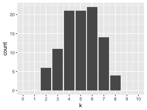
Fair coin
In [2]:
outcomes <- replicate(100, sum(sample(0:1, 10, replace=TRUE)))
In [3]:
options(repr.plot.width=4, repr.plot.height=3)
In [4]:
ggplot(data.frame(k=outcomes), aes(x=k)) +
geom_bar() +
scale_x_continuous(limits=c(0, 10), breaks=0:10)
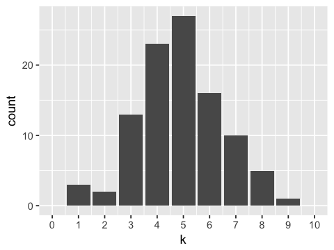
Biased coin
In [5]:
p <- 0.7
outcomes <- replicate(100, sum(sample(0:1, 10, replace=TRUE, prob = c(1-p, p))))
In [6]:
ggplot(data.frame(k=outcomes), aes(x=k)) +
geom_bar() +
scale_x_continuous(limits=c(0, 10), breaks=0:10)

The binomial distribution
The two simulations above are examples of draws from the binomial distribtion. Here we repeat the simulaitons using the more compact binomial distribution model.
Fair coin
In [7]:
outcomes <- rbinom(n=100, size=10, prob=0.5)
In [8]:
ggplot(data.frame(k=outcomes), aes(x=k)) +
geom_bar() +
scale_x_continuous(limits=c(0, 10), breaks=0:10)
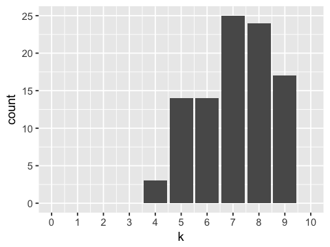
Biased coin
In [9]:
outcomes <- rbinom(n=100, size=10, prob=0.7)
In [10]:
ggplot(data.frame(k=outcomes), aes(x=k)) +
geom_bar() +
scale_x_continuous(limits=c(0, 10), breaks=0:10)
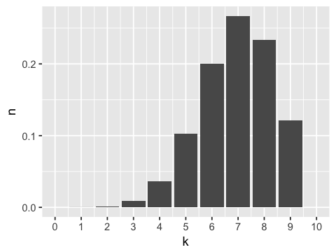
Exact theoretical distribution
In [11]:
k <- 0:10
n <- dbinom(x = k, size =10, prob = 0.7)
In [12]:
ggplot(data.frame(k=k, n=n), aes(x=k, y=n)) +
geom_bar(stat="identity") +
scale_x_continuous(limits=c(0, 10), breaks=0:10)
Exercise 1
Make a histogram of the number of successes expected from 5 trials when the probability of success in each trial is 0.25.
In [ ]:
Exercise 2
You have a miracle drug that will cure 70% of people infected with HIV. You run many clinical trials with 100 HIV-infected people in each trial using this drug. What fraction of the trials have 80 or more people cured?
- Find the answer using properties of the binomial distribution
- Find the answer using a simulation with 10000 trials
In [ ]:
Mean and variance of the binomial distribution
The mean of the binomial distribuiton is \(np\) and the variance is \(np(1-p)\). Note that the mean and variance are defined by the same two parameters \(n\) and \(p\) - once the mean is known, the variance is fixed. Hence it is common for real world data to resemble a binomial distribuiotn except that the variance is larger than expected - this is known as over-dispersion.
In [13]:
n <- 10
p <- 0.7
x <- rbinom(10000, n, p)
In [14]:
mean(x)
In [15]:
round(var(x), 2)
In [16]:
n * p * (1-p)
The Poisson distribution
When the number of trials \(n\) is very large, and the probability of success \(p\) is very small, the binomial distribution can be aproxiated by the simpler Poisson distribution which only has a single parameter \(\lambda = np\).
In [17]:
x <- 0:8
n <- 1000
p <- 0.001
binomial <- dbinom(x, size=n, prob=p)
poisson <-  dpois(x, lambda=n*p)
round(data.frame(x=x, binomial=binomial, poisson=poisson), 4)
| x | binomial | poisson |
|---|---|---|
| 0 | 0.3677 | 0.3679 |
| 1 | 0.3681 | 0.3679 |
| 2 | 0.1840 | 0.1839 |
| 3 | 0.0613 | 0.0613 |
| 4 | 0.0153 | 0.0153 |
| 5 | 0.0030 | 0.0031 |
| 6 | 0.0005 | 0.0005 |
| 7 | 0.0001 | 0.0001 |
| 8 | 0.0000 | 0.0000 |
Exercise 3
Suppose that RNA-seq results in calling errors (e.g. an A is read as a C) once every 1,000 base pairs, and generated single-end reads of exactly 200 base pairs. What fraction of reads would have more than 2 errors?
In [ ]:
Mean and varinace of the Poisson distribuiotn
The mean of the Poisson distribution is \(\lambda\), and its variance is also \(\lambda\). Hence, just as for the binomila distribution, it is common to find real-world data that resembles the Posson distribution, except that the variance is larger than expected. This is another example of over-dispersion.
In [18]:
x <- rpois(10000, 3.14)
In [19]:
round(mean(x), 2)
In [20]:
round(var(x), 2)
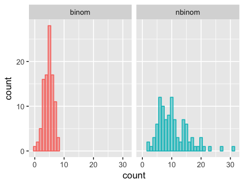
The negative binomial distribution
There are two ways \(k\) successes from a series of \(n\) Bernoulli trials can arise. In the first way, there were \(n\) trials planned, and it just so happened that \(k\) of these were successes. This is modeled by the binomial distribution. However, an alternative scenario is that trials are run until exactly \(k\) successes are observed. This is modeled by the negative binomial distribution.
Note that the nbinom family of functions in R models the number of
failures before a target number of successes is reached, and not the
number of trials.
In [21]:
binom <- rbinom(n=100, size=10, prob=0.5)
nbinom <- rnbinom(n=100, size=10, prob=0.5)
df <- data.frame(binom=binom, nbinom=nbinom)
df <- df %>% gather(dist, count)
In [22]:
ggplot(df, aes(x=count, color=dist, fill=dist)) +
facet_wrap(~ dist) +
geom_bar(alpha=0.5) +
guides(color=F, fill=F)
Utility functions for alternative parameteizations of negative binomial
In [23]:
nb.mean <- function(r, p) {
    r * (1-p)/p
}

nb.var <- function(r, p) {
    r * (1-p)/p^2
}

nb.r <- function(mu, s2) {
    mu^2/(s2 - mu)
}

nb.p <- function(mu, s2) {
    mu/s2
}

nb.disp <- function(mu, s2) {
    (1/mu)*(s2/mu - 1)
}

nb.disp2 <- function(r, p) {
    mu <- nb.mean(r, p)
    s2 <- nb.var(r, p)
    nb.disp(mu, s2)
}
In [24]:
nb.mean(10, 0.5)
In [25]:
nb.var(10, 0.5)
In [26]:
nb.disp2(10, 0.5)
In [27]:
x <- rnbinom(n=100000, size=10, prob=0.5)
In [28]:
round(mean(x), 2)
In [29]:
round(var(x), 2)
Exercise 4
Set \(\lambda = 1\) for the Poisson distribution, and $:raw-latex:mu `= $ for the negative binomial distribution. Compare the two distributions when :math:alpha = 0.001` and \(\alpha = 1.0\).
In [ ]:
The multinomial distribution
The binomial distribtion only allows two outcomes traditionally known as success and failure. The multinomial distiribution generalizes the binomial to allow more than two outcomes.
A common model for the multinomial distribution is that of distributing \(n\) balls to \(k\) urns.
In [30]:
rmultinom(10, size=10, prob=c(1,2,3,4)/10)
| 2 | 1 | 2 | 2 | 1 | 1 | 0 | 2 | 2 | 0 |
| 1 | 2 | 2 | 2 | 2 | 3 | 2 | 1 | 2 | 2 |
| 4 | 1 | 1 | 2 | 3 | 2 | 5 | 5 | 3 | 1 |
| 3 | 6 | 5 | 4 | 4 | 4 | 3 | 2 | 3 | 7 |
Exercise 5
Suppose the genome has 20,000 genes and we sequence 1 million reads. If each read is equally likely to be mapped to any gene
- What is the average number of reads mapped to each gene?
- What is the standard deviation of the number of reads mapped to each gene?
- what is the 95% confidence interval for this estimate of the mean?
In [ ]: