Receiver Operating Characteristic

suppressPackageStartupMessages(library(tidyverse))

Logistic regression concept

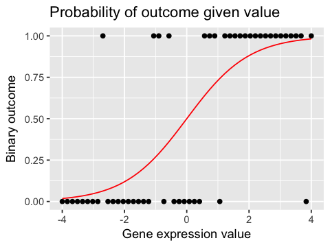
In logistic regression, we want to relate some predictor variable (e..g gene expression value) to the probability of a binary outcome. We would like a linear model since that is mathematically and computationally tractable, but run into the issue that probabilities are restricted to [0,1]. Logistic regression solves this by transforming the output of a linear model into the [0, 1] range.

n <- 50
x <- seq(-4, 4, length.out = n)
a = 0
b = 1

lx <- a + b*x
px <- exp(lx)/(1 + exp(lx))
y <- rbinom(n, 1, px)

df <- data.frame(y=y, x=x, lx=lx, px=px)

options(repr.plot.width=4, repr.plot.height=3)

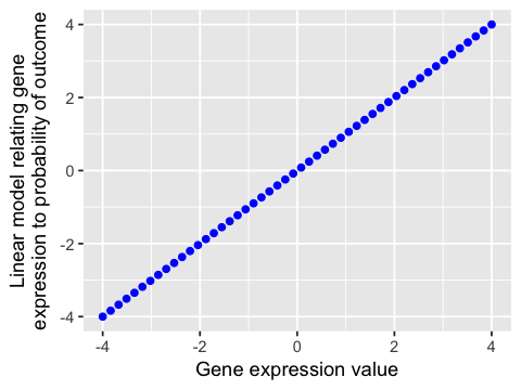
A linear model cannot be directly interpreted as a probability

ggplot(df, aes(x=x, y=lx)) +
geom_point(color='blue') +
labs(x="Gene expression value",
     y="Linear model relating gene\nexpression to probability of outcome")

Data type cannot be displayed:

ggplot(df, aes(x=x, y=y)) +
geom_point() +
geom_line(aes(y=px), color='red') +
labs(x="Gene expression value", y="Binary outcome",
     title="Probability of outcome given value")

Data type cannot be displayed:

Simulation from logistic model

sim.binomial <- function(n, b0, b1, b2, b3) {
    x1 <- rnorm(n)
    x2 <- rnorm(n)
    x3 <- rnorm(n)
    lx <- b0 + b1 * x1 + b2 * x2 + b3 * x3
    px <- exp(lx)/(1 + exp(lx))
    y <- rbinom(n, 1, px)
    data.frame(y, px, x1, x2, x3)
}

LOOCV

set.seed(31219)
data <- sim.binomial(100, 0.1, 0, 1, 0)

head(data)

y	px	x1	x2	x3
0	0.5830298	1.2472628	0.23522348	1.4787281
1	0.4546145	0.5804904	-0.28204321	-0.8217013
1	0.5417889	0.3065363	0.06754626	1.3946841
1	0.8080377	0.4604304	1.33730956	0.6502840
0	0.5436883	1.2094387	0.07519995	0.6585957
1	0.4011430	0.2338796	-0.50070506	-0.8225897

n <- nrow(data)
pred <- numeric(n)
for (i in 1:n) {
    train <- data[-i,]
    test <- data[i,]
    model <- glm(y ~ x1 + x2 + x3, data=train, family="binomial")
    pred[i] <- predict(model, test, type="response")
}
yhat <- ifelse(pred < 0.5, 0, 1)
preddat <- data.frame(probhat=pred, yhat=yhat, y=data$y)

Confusion matrix

suppressPackageStartupMessages(library(caret))

tbl <- table(yhat, data$y)
confusionMatrix(tbl)

Confusion Matrix and Statistics


yhat  0  1
   0 31 26
   1 21 22

               Accuracy : 0.53
                 95% CI : (0.4276, 0.6306)
    No Information Rate : 0.52
    P-Value [Acc > NIR] : 0.4607

                  Kappa : 0.0547
 Mcnemar's Test P-Value : 0.5596

            Sensitivity : 0.5962
            Specificity : 0.4583
         Pos Pred Value : 0.5439
         Neg Pred Value : 0.5116
             Prevalence : 0.5200
         Detection Rate : 0.3100
   Detection Prevalence : 0.5700
      Balanced Accuracy : 0.5272

       'Positive' Class : 0

ROC and AUC

suppressPackageStartupMessages(library(ROCR))

Helper functions

ROC <- function(preddat, mlab = "probhat", ylab = "y") {
    m <- preddat[[mlab]]
    y <- preddat[[ylab]]
    performance(prediction(m, y), measure = "tpr", x.measure = "fpr")
}

AUC <- function(preddat, mlab = "probhat", ylab = "y") {
    m <- preddat[[mlab]]
    y <- preddat[[ylab]]
    performance(prediction(m, y), "auc")@y.values[[1]]
}

Calculate and plot ROC and AUC

my.roc <- ROC(preddat)
my.auc <- AUC(preddat)

my.auc

0.530048076923077

options(repr.plot.width=4, repr.plot.height=4)

plot(my.roc, col = "blue")
abline(0, 1)

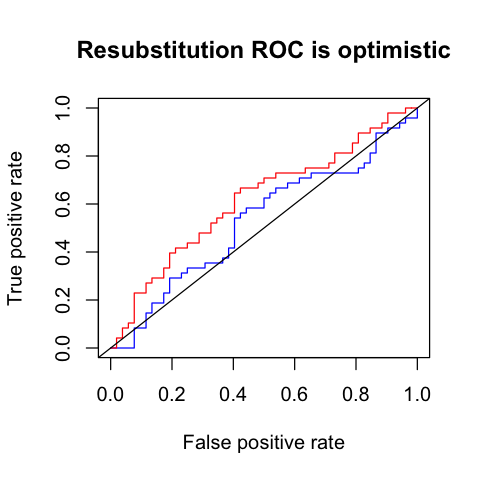
Resubstitution ROC

model.1 <- glm(y ~ x1 + x2 + x3, data=data, family="binomial")
pred.1 <- predict(model.1, type="response")
yhat.1 <- ifelse(pred.1 < 0.5, 0, 1)
preddat.1 <- data.frame(probhat=pred.1, yhat=yhat.1, y=data$y)

rs.roc <- ROC(preddat.1)
rs.auc <- AUC(preddat.1)

rs.auc

0.616987179487179

plot(my.roc, col = "blue", main="Resubstitution ROC is optimistic")
plot(rs.roc, col = "red", add=TRUE)
abline(0, 1)