Computing capstone exercise: Solutions
Data
The data set consists of a simulated (and highly contrived) gene expression levels for 100 subjects. 50 of the subjects are cases, and 50 are controls.
- The expression level of 20,000 genes for each subject is found in a
file
expr-XXX.txtwhereXXXis the subject ID. Missing values are indicated by the stringnan. - The file
cases.txtcontain the IDs of subjects who are in the cases group. - The file
controls.txtcontains the IDs of subjects who are in the controls group. - The file
outcomes.txtcontains the subject ID and blood sugar level for all subjects.
Exercise
Unix shell/command line
For this part - click on the Kernel menu item and select
Change Kernel | Bash
- Download the data from https://www.dropbox.com/s/vivut71p4bkurhw/data.tar.gz
- You will need to quote the URL
In [1]:
wget "https://www.dropbox.com/s/vivut71p4bkurhw/data.tar.gz"
--2017-07-27 10:06:58--  https://www.dropbox.com/s/vivut71p4bkurhw/data.tar.gz
Resolving www.dropbox.com... 162.125.6.1, 2620:100:601c:1::a27d:601
Connecting to www.dropbox.com|162.125.6.1|:443... connected.
HTTP request sent, awaiting response... 302 Found
Location: https://dl.dropboxusercontent.com/content_link/zTZFO6FdHTj3YjweRBYauZZ5YuV5Ej0gsr2rtOUPSdbCs0NQ40ADNWTJMcOm1wGd/file [following]
--2017-07-27 10:06:58--  https://dl.dropboxusercontent.com/content_link/zTZFO6FdHTj3YjweRBYauZZ5YuV5Ej0gsr2rtOUPSdbCs0NQ40ADNWTJMcOm1wGd/file
Resolving dl.dropboxusercontent.com... 162.125.6.6
Connecting to dl.dropboxusercontent.com|162.125.6.6|:443... connected.
HTTP request sent, awaiting response... 200 OK
Length: 3973292 (3.8M) [application/octet-stream]
Saving to: ‘data.tar.gz.1’

data.tar.gz.1       100%[===================>]   3.79M  7.28MB/s    in 0.5s

2017-07-27 10:07:00 (7.28 MB/s) - ‘data.tar.gz.1’ saved [3973292/3973292]
- Regenerate the original data folder from
data.tar.gz
In [2]:
tar -xzf data.tar.gz
- Check if any files have been corrupted using the MDFSUM checksum file and note its
In [3]:
cd data
md5sum -c MD5SUM
cases.txt: OK
controls.txt: OK
expr-1001.txt: OK
expr-1002.txt: OK
expr-1003.txt: OK
expr-1004.txt: OK
expr-1005.txt: OK
expr-1006.txt: OK
expr-1007.txt: OK
expr-1008.txt: OK
expr-1009.txt: OK
expr-1010.txt: OK
expr-1011.txt: OK
expr-1012.txt: OK
expr-1013.txt: OK
expr-1014.txt: OK
expr-1015.txt: OK
expr-1016.txt: OK
expr-1017.txt: OK
expr-1018.txt: OK
expr-1019.txt: OK
expr-1020.txt: OK
expr-1021.txt: OK
expr-1022.txt: OK
expr-1023.txt: OK
expr-1024.txt: OK
expr-1025.txt: OK
expr-1026.txt: OK
expr-1027.txt: OK
expr-1028.txt: OK
expr-1029.txt: OK
expr-1030.txt: OK
expr-1031.txt: OK
expr-1032.txt: OK
expr-1033.txt: OK
expr-1034.txt: OK
expr-1035.txt: OK
expr-1036.txt: OK
expr-1037.txt: OK
expr-1038.txt: OK
expr-1039.txt: OK
expr-1040.txt: OK
expr-1041.txt: OK
expr-1042.txt: OK
expr-1043.txt: OK
expr-1044.txt: OK
expr-1045.txt: OK
expr-1046.txt: OK
expr-1047.txt: OK
expr-1048.txt: OK
expr-1049.txt: OK
expr-1050.txt: OK
expr-1051.txt: OK
expr-1052.txt: OK
expr-1053.txt: OK
expr-1054.txt: OK
expr-1055.txt: OK
expr-1056.txt: OK
expr-1057.txt: OK
expr-1058.txt: OK
expr-1059.txt: OK
expr-1060.txt: OK
expr-1061.txt: OK
expr-1062.txt: OK
expr-1063.txt: OK
expr-1064.txt: OK
expr-1065.txt: OK
expr-1066.txt: OK
expr-1067.txt: OK
expr-1068.txt: OK
expr-1069.txt: OK
expr-1070.txt: OK
expr-1071.txt: OK
expr-1072.txt: OK
expr-1073.txt: OK
expr-1074.txt: FAILED
expr-1075.txt: OK
expr-1076.txt: OK
expr-1077.txt: OK
expr-1078.txt: OK
expr-1079.txt: OK
expr-1080.txt: OK
expr-1081.txt: OK
expr-1082.txt: OK
expr-1083.txt: OK
expr-1084.txt: OK
expr-1085.txt: OK
expr-1086.txt: OK
expr-1087.txt: OK
expr-1088.txt: OK
expr-1089.txt: OK
expr-1090.txt: OK
expr-1091.txt: OK
expr-1092.txt: OK
expr-1093.txt: OK
expr-1094.txt: OK
expr-1095.txt: OK
expr-1096.txt: OK
expr-1097.txt: OK
expr-1098.txt: OK
expr-1099.txt: OK
expr-1100.txt: OK
outcomes.txt: OK
md5sum: WARNING: 1 of 103 computed checksums did NOT match
- Delete the corrupted file and download a correct copy from https://www.dropbox.com/s/vf8qcoj07mcq7wn/FILENAME
- You will need to replace FILENAME with the correct filename
In [4]:
rm expr-1074.txt
wget "https://www.dropbox.com/s/vf8qcoj07mcq7wn/expr-1074.txt"
--2017-07-27 10:07:04--  https://www.dropbox.com/s/vf8qcoj07mcq7wn/expr-1074.txt
Resolving www.dropbox.com... 162.125.6.1, 2620:100:601c:1::a27d:601
Connecting to www.dropbox.com|162.125.6.1|:443... connected.
HTTP request sent, awaiting response... 302 Found
Location: https://dl.dropboxusercontent.com/content_link/GMBFcFrWZQOBq8z3MtOT0haOIcLYErRBgLumqB7oFbhwdCbQbJtKU3kLjf2lArVp/file [following]
--2017-07-27 10:07:05--  https://dl.dropboxusercontent.com/content_link/GMBFcFrWZQOBq8z3MtOT0haOIcLYErRBgLumqB7oFbhwdCbQbJtKU3kLjf2lArVp/file
Resolving dl.dropboxusercontent.com... 162.125.6.6
Connecting to dl.dropboxusercontent.com|162.125.6.6|:443... connected.
HTTP request sent, awaiting response... 200 OK
Length: 111905 (109K) [text/plain]
Saving to: ‘expr-1074.txt’

expr-1074.txt       100%[===================>] 109.28K  --.-KB/s    in 0.03s

2017-07-27 10:07:05 (3.32 MB/s) - ‘expr-1074.txt’ saved [111905/111905]
- Check that there are no
md5sumerrors
In [5]:
md5sum -c MD5SUM
cases.txt: OK
controls.txt: OK
expr-1001.txt: OK
expr-1002.txt: OK
expr-1003.txt: OK
expr-1004.txt: OK
expr-1005.txt: OK
expr-1006.txt: OK
expr-1007.txt: OK
expr-1008.txt: OK
expr-1009.txt: OK
expr-1010.txt: OK
expr-1011.txt: OK
expr-1012.txt: OK
expr-1013.txt: OK
expr-1014.txt: OK
expr-1015.txt: OK
expr-1016.txt: OK
expr-1017.txt: OK
expr-1018.txt: OK
expr-1019.txt: OK
expr-1020.txt: OK
expr-1021.txt: OK
expr-1022.txt: OK
expr-1023.txt: OK
expr-1024.txt: OK
expr-1025.txt: OK
expr-1026.txt: OK
expr-1027.txt: OK
expr-1028.txt: OK
expr-1029.txt: OK
expr-1030.txt: OK
expr-1031.txt: OK
expr-1032.txt: OK
expr-1033.txt: OK
expr-1034.txt: OK
expr-1035.txt: OK
expr-1036.txt: OK
expr-1037.txt: OK
expr-1038.txt: OK
expr-1039.txt: OK
expr-1040.txt: OK
expr-1041.txt: OK
expr-1042.txt: OK
expr-1043.txt: OK
expr-1044.txt: OK
expr-1045.txt: OK
expr-1046.txt: OK
expr-1047.txt: OK
expr-1048.txt: OK
expr-1049.txt: OK
expr-1050.txt: OK
expr-1051.txt: OK
expr-1052.txt: OK
expr-1053.txt: OK
expr-1054.txt: OK
expr-1055.txt: OK
expr-1056.txt: OK
expr-1057.txt: OK
expr-1058.txt: OK
expr-1059.txt: OK
expr-1060.txt: OK
expr-1061.txt: OK
expr-1062.txt: OK
expr-1063.txt: OK
expr-1064.txt: OK
expr-1065.txt: OK
expr-1066.txt: OK
expr-1067.txt: OK
expr-1068.txt: OK
expr-1069.txt: OK
expr-1070.txt: OK
expr-1071.txt: OK
expr-1072.txt: OK
expr-1073.txt: OK
expr-1074.txt: OK
expr-1075.txt: OK
expr-1076.txt: OK
expr-1077.txt: OK
expr-1078.txt: OK
expr-1079.txt: OK
expr-1080.txt: OK
expr-1081.txt: OK
expr-1082.txt: OK
expr-1083.txt: OK
expr-1084.txt: OK
expr-1085.txt: OK
expr-1086.txt: OK
expr-1087.txt: OK
expr-1088.txt: OK
expr-1089.txt: OK
expr-1090.txt: OK
expr-1091.txt: OK
expr-1092.txt: OK
expr-1093.txt: OK
expr-1094.txt: OK
expr-1095.txt: OK
expr-1096.txt: OK
expr-1097.txt: OK
expr-1098.txt: OK
expr-1099.txt: OK
expr-1100.txt: OK
outcomes.txt: OK
Data munging
For this part - click on the Kernel menu item and select
Change Kernel | R
- Create a
data.framecalledexprwhere each row represents a gene, and each column represents a subject. Give meaningful row names of the formgeneX(where X goes from 1:20000) andptX(where X goes from 1001:1100, using the PID in the filename). - When loading the files, make sure you also handle missing data indicated by the string ‘nan’ correctly.
In [186]:
suppressPackageStartupMessages(library(tidyverse))
In [187]:
files <- paste('data/', 'expr-', 1001:1100, '.txt', sep='')
In [188]:
data <- lapply(files, read.table)
In [189]:
expr <- bind_cols(data)
In [190]:
dim(expr)
- 20000
- 100
In [191]:
rownames(expr) = paste('gene', 1:nrow(expr), sep='')
In [192]:
colnames(expr) = paste('pt', 1001:1100, sep='')
In [193]:
head(expr)
| pt1001 | pt1002 | pt1003 | pt1004 | pt1005 | pt1006 | pt1007 | pt1008 | pt1009 | pt1010 | ⋯ | pt1091 | pt1092 | pt1093 | pt1094 | pt1095 | pt1096 | pt1097 | pt1098 | pt1099 | pt1100 | |
|---|---|---|---|---|---|---|---|---|---|---|---|---|---|---|---|---|---|---|---|---|---|
| gene1 | 8.39 | 3.60 | 12.55 | -2.15 | -8.04 | -10.42 | -4.39 | -1.82 | 7.38 | 5.70 | ⋯ | -6.29 | -3.52 | -4.81 | 0.37 | -2.22 | -4.14 | 7.40 | -1.34 | -3.34 | 5.17 |
| gene2 | 0.63 | 6.18 | 8.35 | 9.87 | -4.97 | 0.86 | -3.28 | -4.73 | -14.21 | -7.32 | ⋯ | 4.05 | 2.45 | -1.42 | 2.29 | -3.84 | -6.12 | -2.89 | -5.94 | 15.15 | 12.76 |
| gene3 | 1.40 | 9.47 | 2.42 | -1.58 | -8.86 | -2.05 | -1.31 | -1.64 | 9.68 | -3.50 | ⋯ | -4.38 | 0.96 | 5.34 | 7.45 | -6.63 | 4.84 | -3.58 | -8.33 | 3.76 | -7.13 |
| gene4 | 1.44 | -2.81 | 4.60 | 1.22 | 4.14 | 10.04 | -0.99 | 12.57 | -7.22 | -7.75 | ⋯ | -5.44 | 3.74 | -6.08 | 1.96 | -2.47 | 0.66 | 7.34 | -7.44 | 1.48 | 6.83 |
| gene5 | -0.38 | 0.46 | 0.41 | -12.49 | -11.06 | 3.19 | -4.40 | 3.55 | -9.26 | 1.63 | ⋯ | 1.80 | 4.17 | -7.01 | 0.80 | 2.02 | 0.30 | 3.85 | -7.74 | 9.59 | 6.05 |
| gene6 | -8.52 | 5.84 | 1.56 | -1.52 | 4.73 | 5.90 | -5.81 | -0.16 | -0.62 | 0.91 | ⋯ | 9.14 | -9.82 | 7.51 | -11.27 | -2.70 | -0.78 | 3.66 | 10.58 | 7.58 | 14.13 |
- Remove any gene(row) whose values are all zero. How many genes were dropped?
In [194]:
idx <- rowSums(abs(expr)) == 0
expr <- expr[!idx,]
In [195]:
dim(expr)
- 19998
- 100
- Remove any genes (row) with missing data. How many genes were dropped?
In [196]:
expr <- expr %>% drop_na()
In [197]:
dim(expr)
- 19993
- 100
- Scale all genes to have zero mean and unit standard deviation
In [198]:
expr <- t(scale(t(expr)))
In [199]:
head(round(apply(expr, 1, sd), 2), 3)
- gene1
- 1
- gene2
- 1
- gene3
- 1
In [200]:
head(round(apply(expr, 1, mean), 2), 3)
- gene1
- 0
- gene2
- 0
- gene3
- 0
- Create a data frame
groupwith two columnsPIDandGroupthat indicates whether each patient is a case or control. Use the information from thecases.txtandcontrols.txtfiles.
In [201]:
cases <- read.table('data/cases.txt')
ctrls <- read.table('data/controls.txt')
In [202]:
n1 <- nrow(cases)
n2 <- nrow(ctrls)
In [203]:
grp <- c(rep('case', n1), rep('ctrl', n2))
In [204]:
group <- data.frame(PID=bind_rows(cases, ctrls), grp)
In [205]:
colnames(group) <- c('PID', 'Group')
In [206]:
head(group, 3)
| PID | Group |
|---|---|
| 1088 | case |
| 1022 | case |
| 1064 | case |
In [207]:
tail(group, 3)
| PID | Group | |
|---|---|---|
| 98 | 1096 | ctrl |
| 99 | 1072 | ctrl |
| 100 | 1038 | ctrl |
Unsupervised Learning
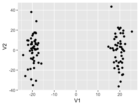
- Use classic MDS (multi-dimensional scaling) to embed the data in 2D
and make a scatter plot with
ggplot2
In [208]:
mds <- as.data.frame(cmdscale(dist(t(expr)), k=2))
In [209]:
str(mds)
'data.frame':   100 obs. of  2 variables:
 $ V1: num  -19.5 21.9 19.5 -22 -21.1 ...
 $ V2: num  -7.44 13.636 -36.314 5.243 -0.752 ...
In [210]:
options(repr.plot.width=4, repr.plot.height=3)
In [211]:
ggplot(mds, aes(x=V1, y=V2)) + geom_point()
Data type cannot be displayed:
- Use a t-test to find all genes differentially expressed in the cases
and controls group with a False Discovery Rate (FDR) of 0.05 using
the Benjamini–Hochberg (BH) procedure. Save the filtered genes in a
data.framecalledhits.
In [212]:
suppressPackageStartupMessages(library(genefilter))
In [213]:
head(group, 3)
| PID | Group |
|---|---|
| 1088 | case |
| 1022 | case |
| 1064 | case |
In [214]:
group <- group %>% arrange(PID)
head(group)
| PID | Group |
|---|---|
| 1001 | case |
| 1002 | ctrl |
| 1003 | ctrl |
| 1004 | case |
| 1005 | case |
| 1006 | case |
In [215]:
dim(expr)
- 19993
- 100
In [216]:
p.values <- rowttests(expr, fac = group$Group)$p.value
In [217]:
head(p.values)
- 0.810340264500016
- 0.0204475853560852
- 0.233159743584127
- 0.412635280852636
- 0.165387577174332
- 0.933613549615968
In [218]:
p.bh <- p.adjust(p.values, method='BH')
In [219]:
idx <- p.bh < 0.01
In [220]:
hits <- expr[idx,]
rownames(hits)
- 'gene160'
- 'gene393'
- 'gene412'
- 'gene439'
- 'gene452'
- 'gene490'
- 'gene506'
- 'gene601'
- 'gene683'
- 'gene748'
- 'gene766'
- 'gene771'
- 'gene808'
- 'gene830'
- 'gene834'
- 'gene862'
- 'gene888'
- 'gene914'
- 'gene1013'
- 'gene1035'
- 'gene1057'
- 'gene1082'
- 'gene1138'
- 'gene1172'
- 'gene1194'
- 'gene1322'
- 'gene1338'
- 'gene1462'
- 'gene1563'
- 'gene1582'
- 'gene1594'
- 'gene1775'
- 'gene1844'
- 'gene1857'
- 'gene1868'
- 'gene1910'
- 'gene1950'
- 'gene1957'
- 'gene2094'
- 'gene2106'
- 'gene2119'
- 'gene2148'
- 'gene2233'
- 'gene2253'
- 'gene2300'
- 'gene2358'
- 'gene2407'
- 'gene2450'
- 'gene2454'
- 'gene2461'
- 'gene2508'
- 'gene2548'
- 'gene2560'
- 'gene2608'
- 'gene2630'
- 'gene2642'
- 'gene2671'
- 'gene2736'
- 'gene2772'
- 'gene2818'
- 'gene2822'
- 'gene2941'
- 'gene2971'
- 'gene3012'
- 'gene3072'
- 'gene3116'
- 'gene3215'
- 'gene3262'
- 'gene3269'
- 'gene3306'
- 'gene3403'
- 'gene3455'
- 'gene3490'
- 'gene3492'
- 'gene3546'
- 'gene3574'
- 'gene3647'
- 'gene3693'
- 'gene3731'
- 'gene3748'
- 'gene3769'
- 'gene3802'
- 'gene3964'
- 'gene3971'
- 'gene4007'
- 'gene4028'
- 'gene4059'
- 'gene4097'
- 'gene4117'
- 'gene4233'
- 'gene4293'
- 'gene4427'
- 'gene4438'
- 'gene4501'
- 'gene4527'
- 'gene4634'
- 'gene4652'
- 'gene4723'
- 'gene4846'
- 'gene4890'
- 'gene5212'
- 'gene5233'
- 'gene5272'
- 'gene5375'
- 'gene5478'
- 'gene5520'
- 'gene5664'
- 'gene5770'
- 'gene5828'
- 'gene5936'
- 'gene5975'
- 'gene5987'
- 'gene6025'
- 'gene6029'
- 'gene6096'
- 'gene6097'
- 'gene6102'
- 'gene6104'
- 'gene6210'
- 'gene6412'
- 'gene6478'
- 'gene6534'
- 'gene6650'
- 'gene6672'
- 'gene6678'
- 'gene6756'
- 'gene6779'
- 'gene6908'
- 'gene7116'
- 'gene7123'
- 'gene7215'
- 'gene7220'
- 'gene7250'
- 'gene7252'
- 'gene7363'
- 'gene7374'
- 'gene7496'
- 'gene7568'
- 'gene7578'
- 'gene7648'
- 'gene7692'
- 'gene7704'
- 'gene7713'
- 'gene7766'
- 'gene7783'
- 'gene7873'
- 'gene8102'
- 'gene8163'
- 'gene8304'
- 'gene8559'
- 'gene8758'
- 'gene8843'
- 'gene8906'
- 'gene8924'
- 'gene8993'
- 'gene8995'
- 'gene9104'
- 'gene9192'
- 'gene9203'
- 'gene9227'
- 'gene9326'
- 'gene9403'
- 'gene9506'
- 'gene9516'
- 'gene9652'
- 'gene9653'
- 'gene9679'
- 'gene9725'
- 'gene9741'
- 'gene9817'
- 'gene9834'
- 'gene9848'
- 'gene9857'
- 'gene9906'
- 'gene10003'
- 'gene10057'
- 'gene10105'
- 'gene10119'
- 'gene10190'
- 'gene10210'
- 'gene10211'
- 'gene10283'
- 'gene10326'
- 'gene10437'
- 'gene10446'
- 'gene10529'
- 'gene10587'
- 'gene10639'
- 'gene10657'
- 'gene10667'
- 'gene10674'
- 'gene10682'
- 'gene10696'
- 'gene10706'
- 'gene10737'
- 'gene10778'
- 'gene10812'
- 'gene10876'
- 'gene10918'
- 'gene10949'
- 'gene10956'
- 'gene11212'
- 'gene11218'
- 'gene11295'
- 'gene11357'
- 'gene11360'
- 'gene11366'
- 'gene11384'
- 'gene11429'
- 'gene11433'
- 'gene11478'
- 'gene11527'
- 'gene11553'
- 'gene11564'
- 'gene11631'
- 'gene11824'
- 'gene11931'
- 'gene12102'
- 'gene12211'
- 'gene12253'
- 'gene12354'
- 'gene12370'
- 'gene12377'
- 'gene12425'
- 'gene12508'
- 'gene12547'
- 'gene12559'
- 'gene12567'
- 'gene12674'
- 'gene12675'
- 'gene12694'
- 'gene12704'
- 'gene12723'
- 'gene12769'
- 'gene12777'
- 'gene12809'
- 'gene12819'
- 'gene12825'
- 'gene12864'
- 'gene12902'
- 'gene12927'
- 'gene12947'
- 'gene13148'
- 'gene13170'
- 'gene13179'
- 'gene13233'
- 'gene13381'
- 'gene13461'
- 'gene13567'
- 'gene13607'
- 'gene13649'
- 'gene13711'
- 'gene13723'
- 'gene13742'
- 'gene13780'
- 'gene13823'
- 'gene13832'
- 'gene13872'
- 'gene14038'
- 'gene14154'
- 'gene14161'
- 'gene14178'
- 'gene14434'
- 'gene14443'
- 'gene14508'
- 'gene14539'
- 'gene14560'
- 'gene14590'
- 'gene14604'
- 'gene14623'
- 'gene14656'
- 'gene14660'
- 'gene14782'
- 'gene14784'
- 'gene14808'
- 'gene14889'
- 'gene14924'
- 'gene15062'
- 'gene15069'
- 'gene15083'
- 'gene15087'
- 'gene15101'
- 'gene15128'
- 'gene15173'
- 'gene15177'
- 'gene15180'
- 'gene15232'
- 'gene15263'
- 'gene15361'
- 'gene15415'
- 'gene15454'
- 'gene15523'
- 'gene15530'
- 'gene15592'
- 'gene15596'
- 'gene15619'
- 'gene15709'
- 'gene15714'
- 'gene15725'
- 'gene15743'
- 'gene15892'
- 'gene16056'
- 'gene16088'
- 'gene16095'
- 'gene16122'
- 'gene16164'
- 'gene16197'
- 'gene16213'
- 'gene16240'
- 'gene16256'
- 'gene16482'
- 'gene16647'
- 'gene16701'
- 'gene16705'
- 'gene16788'
- 'gene16810'
- 'gene16830'
- 'gene16870'
- 'gene16967'
- 'gene16978'
- 'gene16987'
- 'gene17113'
- 'gene17129'
- 'gene17146'
- 'gene17224'
- 'gene17233'
- 'gene17396'
- 'gene17432'
- 'gene17562'
- 'gene17582'
- 'gene17605'
- 'gene17625'
- 'gene17862'
- 'gene17910'
- 'gene18009'
- 'gene18055'
- 'gene18169'
- 'gene18206'
- 'gene18207'
- 'gene18316'
- 'gene18329'
- 'gene18341'
- 'gene18375'
- 'gene18410'
- 'gene18453'
- 'gene18487'
- 'gene18509'
- 'gene18530'
- 'gene18722'
- 'gene18811'
- 'gene18847'
- 'gene18905'
- 'gene18957'
- 'gene19008'
- 'gene19066'
- 'gene19080'
- 'gene19086'
- 'gene19137'
- 'gene19216'
- 'gene19251'
- 'gene19287'
- 'gene19564'
- 'gene19666'
- 'gene19701'
- 'gene19757'
- 'gene19771'
- 'gene19795'
- 'gene19930'
- 'gene19978'
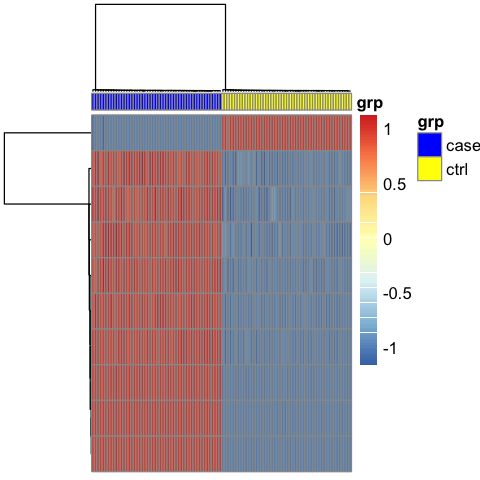
- Plot a heatmap of the genes that meet the FDR filter using agglomerative hierarchical clustering with complete linkage for the dendrograms. Arrange the subjects so all controls are on the left and all cases are on the right in the heatmap.
In [221]:
clusters <- hclust(dist(hits), method = 'complete')
In [222]:
library(pheatmap)
In [223]:
annot <- data.frame(grp=group$Group, row.names=colnames(hits))
In [224]:
options(repr.plot.width=8, repr.plot.height=8)
In [303]:
pheatmap(hits,
         clustering_method = 'single',
         annotation_col = annot,
         annotation_colors = list(grp = c(case = "blue", ctrl = "yellow")),
         show_rownames = FALSE, show_colnames = FALSE,
        )
Supervised Learning
- Perform logistic regression using LOOCV and the top 10 genes to generate class predictions (case or control) for all subjects
In [226]:
n <- nrow(df)
pred <- numeric(n)
for (i in 1:n) {
    p.values <- rowttests(expr[,-i], fac = group$Group[-i])$p.value
    idx <- order(p.values)
    hits <- expr[idx[1:10],]

    # transpose so geens are variables then add group informaiton
    df <- t(hits)
    df <- data.frame(y=as.factor(group$Group), df)

    model <- glm(y ~ ., data=df[-i,], family='binomial')
    pred[i] <- predict(model, df[i,], type='response')
}
yhat <- ifelse(pred < 0.5, 1, 2)
- Evaluate the accuracy, sensitivity, specificity, PPV, NPV of the LOOCV logistic regression
In [227]:
suppressPackageStartupMessages(library(caret))
In [228]:
confusionMatrix(yhat, as.integer(group$Group))
Confusion Matrix and Statistics

          Reference
Prediction  1  2
         1 50  0
         2  0 50

               Accuracy : 1
                 95% CI : (0.9638, 1)
    No Information Rate : 0.5
    P-Value [Acc > NIR] : < 2.2e-16

                  Kappa : 1
 Mcnemar's Test P-Value : NA

            Sensitivity : 1.0
            Specificity : 1.0
         Pos Pred Value : 1.0
         Neg Pred Value : 1.0
             Prevalence : 0.5
         Detection Rate : 0.5
   Detection Prevalence : 0.5
      Balanced Accuracy : 1.0

       'Positive' Class : 1
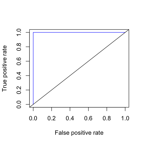
- Plot an ROC curve for the LOOCV predictions
In [229]:
suppressPackageStartupMessages(library(ROCR))
In [230]:
ROC <- function(preddat, mlab = "probhat", ylab = "y") {
    m <- preddat[[mlab]]
    y <- preddat[[ylab]]
    performance(prediction(m, y), measure = "tpr", x.measure = "fpr")
}
In [231]:
preddat <- data.frame(probhat=pred, yhat=yhat, y=as.integer(group$Group))
my.roc <- ROC(preddat)
In [232]:
options(repr.plot.width=4, repr.plot.height=4)
In [233]:
plot(my.roc, col = "blue")
abline(0, 1)
- Read the
outcomes.txtdata into adata.framecalledoutcomeswith two columnsPIDandoutcome.
In [234]:
outcomes <- read.table('data/outcomes.txt')
In [235]:
head(outcomes)
| V1 | V2 |
|---|---|
| 1035 | 491.65 |
| 1091 | 512.43 |
| 1095 | 513.15 |
| 1019 | 571.56 |
| 1081 | 517.13 |
| 1077 | 535.44 |
In [236]:
colnames(outcomes) = c('PID', 'outcome')
In [243]:
outcomes$PID = as.factor(outcomes$PID)
In [244]:
head(outcomes)
| PID | outcome |
|---|---|
| 1035 | 491.65 |
| 1091 | 512.43 |
| 1095 | 513.15 |
| 1019 | 571.56 |
| 1081 | 517.13 |
| 1077 | 535.44 |
- Merge the
outcomesandexprby joining on thePIDcolumn.
In [239]:
head(data)
| PID | gene1 | gene2 | gene3 | gene4 | gene5 | gene6 | gene7 | gene8 | gene9 | ⋯ | gene19991 | gene19992 | gene19993 | gene19994 | gene19995 | gene19996 | gene19997 | gene19998 | gene19999 | gene20000 |
|---|---|---|---|---|---|---|---|---|---|---|---|---|---|---|---|---|---|---|---|---|
| pt1001 | 1.5619416 | 0.1274296 | 0.3818537 | 0.1754658 | -0.119502825 | -1.40226660 | -0.8833635 | -0.94309346 | -0.4272967 | ⋯ | -0.62969491 | 0.2422296 | 0.8998351 | 0.6209216 | -0.4764382 | -0.08677132 | -0.8747234 | 0.5187669 | 0.2592983 | -0.2476950 |
| pt1002 | 0.7334951 | 0.8649770 | 1.8528351 | -0.5721328 | 0.012561868 | 0.54493040 | 0.5795712 | 0.06164405 | -0.5987428 | ⋯ | 0.37135403 | 0.8149647 | 0.9313236 | -0.1974330 | -1.5460305 | 0.43927981 | 0.1554110 | -0.4076643 | -1.3342893 | -0.1228203 |
| pt1003 | 2.2814275 | 1.1533513 | 0.5677770 | 0.7313274 | 0.004700874 | -0.03543193 | -0.9456161 | -1.74386169 | 1.6602020 | ⋯ | 0.93993227 | -0.6044223 | 0.1441122 | 1.1243218 | -0.2946378 | -1.49409366 | -0.1392395 | 1.0223122 | 0.7461696 | 1.3233091 |
| pt1004 | -0.2609866 | 1.3553463 | -0.1613340 | 0.1367666 | -2.023435482 | -0.45307586 | -0.4475958 | 0.96817412 | -1.0207642 | ⋯ | 0.63478797 | -1.6004834 | 0.2385775 | 0.4706923 | -2.1459718 | 1.00600499 | 1.1101697 | -1.0333510 | -0.9573566 | 0.8587216 |
| pt1005 | -1.2796818 | -0.6167624 | -1.4883161 | 0.6504108 | -1.798611064 | 0.39441587 | -0.3542170 | -0.33118565 | -0.2219380 | ⋯ | 0.06840501 | 0.5348225 | -0.3387108 | 0.2914713 | 0.9537248 | 1.61069262 | -0.7970636 | 1.7090697 | -0.3343707 | -1.0479672 |
| pt1006 | -1.6913107 | 0.1579946 | -0.2470046 | 1.6882536 | 0.441772120 | 0.55306632 | 1.2643491 | 1.61029959 | 0.9706492 | ⋯ | -0.83824677 | -1.2207351 | -0.2862301 | 1.4972595 | -0.8763991 | -2.01472158 | 0.2444913 | -0.3154821 | -0.8359005 | 0.8976610 |
In [241]:
head(outcomes)
| PID | outcome |
|---|---|
| 1035 | 491.65 |
| 1091 | 512.43 |
| 1095 | 513.15 |
| 1019 | 571.56 |
| 1081 | 517.13 |
| 1077 | 535.44 |
In [246]:
data <- data.frame(t(expr)) %>% rownames_to_column('PID') %>% mutate(PID=as.factor(substr(PID, 3,6)))
df <- inner_join(data, outcomes, by='PID')
- Perform LOOCV linear regression using the 5 genes most correlated with outcome to get outcome predictions for each subject
In [260]:
head(df, 2)
| gene1 | gene2 | gene3 | gene4 | gene5 | gene6 | gene7 | gene8 | gene9 | gene10 | ⋯ | gene19992 | gene19993 | gene19994 | gene19995 | gene19996 | gene19997 | gene19998 | gene19999 | gene20000 | outcome | |
|---|---|---|---|---|---|---|---|---|---|---|---|---|---|---|---|---|---|---|---|---|---|
| 1001 | 1.5619416 | 0.1274296 | 0.3818537 | 0.1754658 | -0.11950283 | -1.4022666 | -0.8833635 | -0.94309346 | -0.4272967 | 0.3923721 | ⋯ | 0.2422296 | 0.8998351 | 0.6209216 | -0.4764382 | -0.08677132 | -0.8747234 | 0.5187669 | 0.2592983 | -0.2476950 | 629.10 |
| 1002 | 0.7334951 | 0.8649770 | 1.8528351 | -0.5721328 | 0.01256187 | 0.5449304 | 0.5795712 | 0.06164405 | -0.5987428 | 0.3893356 | ⋯ | 0.8149647 | 0.9313236 | -0.1974330 | -1.5460305 | 0.43927981 | 0.1554110 | -0.4076643 | -1.3342893 | -0.1228203 | 558.71 |
In [259]:
df <- df %>% column_to_rownames(var='PID')
In [282]:
df %>% select(outcome) %>% head
| outcome | |
|---|---|
| 1001 | 629.10 |
| 1002 | 558.71 |
| 1003 | 583.89 |
| 1004 | 482.18 |
| 1005 | 403.61 |
| 1006 | 512.62 |
In [292]:
n <- nrow(df)
pred <- numeric(n)
for (i in 1:n) {
    y <- df$outcome
    x <- df[, -ncol(df)]

    r <- abs(cor(y[-i], x[-i,]))
    idx <- order(desc(r))[1:5]

    data <- data.frame(y=y, x=x[, idx])
    model <- lm(y ~ ., data=data[-i,])
    pred[i] <- predict(model, data[i,])
}
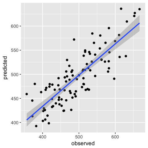
- Plot a scatter plot with a linear regression curve for predicted (y)
versus observed (x) values using
ggplot2
In [293]:
df.1 <- data.frame(observed=df$outcome, predicted=pred)
In [298]:
ggplot(df.1, aes(x=observed, y=predicted)) +
geom_point() +
geom_smooth(method='lm')
Data type cannot be displayed:
In [ ]: