DESeq2 Analysis of 2015 Data

In this notebook, we will reproduce the dendrograms from the 2015 data shown in the welcome slides

Load packages

Load requisite R packages.

library(DESeq2)
library(tools)
library(dendextend)
library(dplyr)
library(RColorBrewer)
options(width=100)

Loading required package: S4Vectors
Loading required package: stats4
Loading required package: BiocGenerics
Loading required package: parallel

Attaching package: ‘BiocGenerics’

The following objects are masked from ‘package:parallel’:

    clusterApply, clusterApplyLB, clusterCall, clusterEvalQ,
    clusterExport, clusterMap, parApply, parCapply, parLapply,
    parLapplyLB, parRapply, parSapply, parSapplyLB

The following objects are masked from ‘package:stats’:

    IQR, mad, xtabs

The following objects are masked from ‘package:base’:

    anyDuplicated, append, as.data.frame, cbind, colnames, do.call,
    duplicated, eval, evalq, Filter, Find, get, grep, grepl, intersect,
    is.unsorted, lapply, lengths, Map, mapply, match, mget, order,
    paste, pmax, pmax.int, pmin, pmin.int, Position, rank, rbind,
    Reduce, rownames, sapply, setdiff, sort, table, tapply, union,
    unique, unsplit, which, which.max, which.min


Attaching package: ‘S4Vectors’

The following objects are masked from ‘package:base’:

    colMeans, colSums, expand.grid, rowMeans, rowSums

Loading required package: IRanges
Loading required package: GenomicRanges
Loading required package: GenomeInfoDb
Loading required package: SummarizedExperiment
Loading required package: Biobase
Welcome to Bioconductor

    Vignettes contain introductory material; view with
    'browseVignettes()'. To cite Bioconductor, see
    'citation("Biobase")', and for packages 'citation("pkgname")'.


---------------------
Welcome to dendextend version 1.5.2
Type citation('dendextend') for how to cite the package.

Type browseVignettes(package = 'dendextend') for the package vignette.
The github page is: https://github.com/talgalili/dendextend/

Suggestions and bug-reports can be submitted at: https://github.com/talgalili/dendextend/issues
Or contact: <tal.galili@gmail.com>

        To suppress this message use:  suppressPackageStartupMessages(library(dendextend))
---------------------


Attaching package: ‘dendextend’

The following object is masked from ‘package:stats’:

    cutree


Attaching package: ‘dplyr’

The following object is masked from ‘package:Biobase’:

    combine

The following objects are masked from ‘package:GenomicRanges’:

    intersect, setdiff, union

The following object is masked from ‘package:GenomeInfoDb’:

    intersect

The following objects are masked from ‘package:IRanges’:

    collapse, desc, intersect, regroup, setdiff, slice, union

The following objects are masked from ‘package:S4Vectors’:

    first, intersect, rename, setdiff, setequal, union

The following objects are masked from ‘package:BiocGenerics’:

    combine, intersect, setdiff, union

The following objects are masked from ‘package:stats’:

    filter, lag

The following objects are masked from ‘package:base’:

    intersect, setdiff, setequal, union

Prepare for Data Import

First set the directory under which the HTSeq count files are stored

datadir<-"~/work/HTS_SummerCourse_2017/Materials/Statistics/08032017/Data/2015"

Next, put the filenames into a data frame

phdata<-data.frame(fname=list.files(path=datadir,pattern="*.csv"),stringsAsFactors=FALSE)

It is always a good idea to check the dimension of the file you have read in

dim(phdata)

1. 30
2. 1

Extract the label from the filename.

phdata <- phdata %>% transmute(sample=substr(fname,1,4),fname)

Add some design info to the data frame. We will add the treatment factor (the first character of the sample string: 7 or 8), the replicate id (the second character in the

Note that tools::md5sum will add the MD5 signature for each of the HTSeq count files. You should keep track of these for the purpose of conducting reproducible analysis

phdata <- phdata %>%
                mutate(trt=as.factor(substr(sample,1,1)),
                       repl=substr(sample,2,2),
                       team=substr(sample,4,4),
                       md5=tools::md5sum(file.path(datadir,fname)))
head(phdata)

	sample	fname	trt	repl	team	md5
1	7A_E	7A_E.csv	7	A	E	NA
2	7A_G	7A_G.csv	7	A	G	NA
3	7A_K	7A_K.csv	7	A	K	NA
4	7A_N	7A_N.csv	7	A	N	NA
5	7A_P	7A_P.csv	7	A	P	NA
6	7B_E	7B_E.csv	7	B	E	NA

Now, we import the counts. Note that the first argument is the sample table while the second is the directory storing the count files. The last argument specifies the design. More on this later.

dds<-DESeqDataSetFromHTSeqCount(sampleTable=phdata,directory=datadir,design=~ trt)

Estimate library specific size factors and gene specific dispersion paramaters

Estimate Size factors

dds<-estimateSizeFactors(dds)

Estimate dispersion parameters

dds<-estimateDispersions(dds)

gene-wise dispersion estimates
mean-dispersion relationship
final dispersion estimates

Inspect object

dds

class: DESeqDataSet
dim: 4444 30
metadata(1): version
assays(2): counts mu
rownames(4444): gene0 gene1 ... gene998 gene999
rowData names(9): baseMean baseVar ... dispOutlier dispMAP
colnames(30): 7A_E 7A_G ... 8C_N 8C_P
colData names(5): trt repl team md5 sizeFactor

Create dendrograms

For this tutorial, we will use t he expression data based on rlog transformation.

rlogexp<-assay(rlog(dds))

Next, we create the dendrogram object using hierarchical clustering using complete linkage (method=”complete”).

Note that you have you transpose the expression matrix as R assumes that the samples are along the rows and that the genes are across the columns. This is accomplished using the t() function. Next, you create the distance matrix for this expression matrix using the dist() function. Afterwards, you conduct hierachical clustering on the basis of complete linkage using this distance matrix usin the dist() function. Finally, the results from the clustering is converted into a dendrogram class using the as.dendrogram() function

dend <- rlogexp %>%
                t %>%
                dist %>%
                hclust(method="complete") %>%
                as.dendrogram

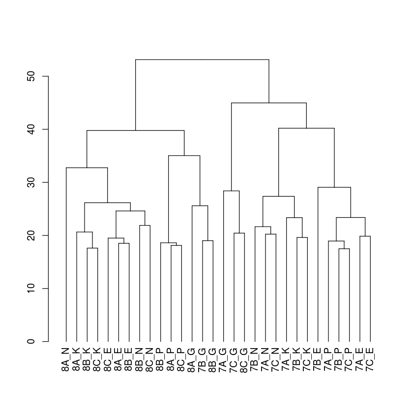
Let’s look as a plot

dend %>% plot

Next, we will add some eye candy to this dendrogram. We will add the treatment label as symbols and the group/team labels as colors. Note that one can extract the labels from the dendrogram using the labels() function

labels(dend)

1. '8A_N'
2. '8A_K'
3. '8B_K'
4. '8C_K'
5. '8C_E'
6. '8A_E'
7. '8B_E'
8. '8B_N'
9. '8C_N'
10. '8B_P'
11. '8A_P'
12. '8C_P'
13. '8A_G'
14. '7B_G'
15. '8B_G'
16. '7A_G'
17. '7C_G'
18. '8C_G'
19. '7B_N'
20. '7A_N'
21. '7C_N'
22. '7A_K'
23. '7B_K'
24. '7C_K'
25. '7B_E'
26. '7A_P'
27. '7B_P'
28. '7C_P'
29. '7A_E'
30. '7C_E'

Now use this information to create a treatment label vector

trtlab<-c(2,19)[factor(substr(labels(dend),1,1))]
trtlab

1. 19
2. 19
3. 19
4. 19
5. 19
6. 19
7. 19
8. 19
9. 19
10. 19
11. 19
12. 19
13. 19
14. 2
15. 19
16. 2
17. 2
18. 19
19. 2
20. 2
21. 2
22. 2
23. 2
24. 2
25. 2
26. 2
27. 2
28. 2
29. 2
30. 2

and then a group label vector

grplab<-brewer.pal(5,"Set1")[factor(substr(labels(dend),4,4))]
grplab

1. '#984EA3'
2. '#4DAF4A'
3. '#4DAF4A'
4. '#4DAF4A'
5. '#E41A1C'
6. '#E41A1C'
7. '#E41A1C'
8. '#984EA3'
9. '#984EA3'
10. '#FF7F00'
11. '#FF7F00'
12. '#FF7F00'
13. '#377EB8'
14. '#377EB8'
15. '#377EB8'
16. '#377EB8'
17. '#377EB8'
18. '#377EB8'
19. '#984EA3'
20. '#984EA3'
21. '#984EA3'
22. '#4DAF4A'
23. '#4DAF4A'
24. '#4DAF4A'
25. '#E41A1C'
26. '#FF7F00'
27. '#FF7F00'
28. '#FF7F00'
29. '#E41A1C'
30. '#E41A1C'

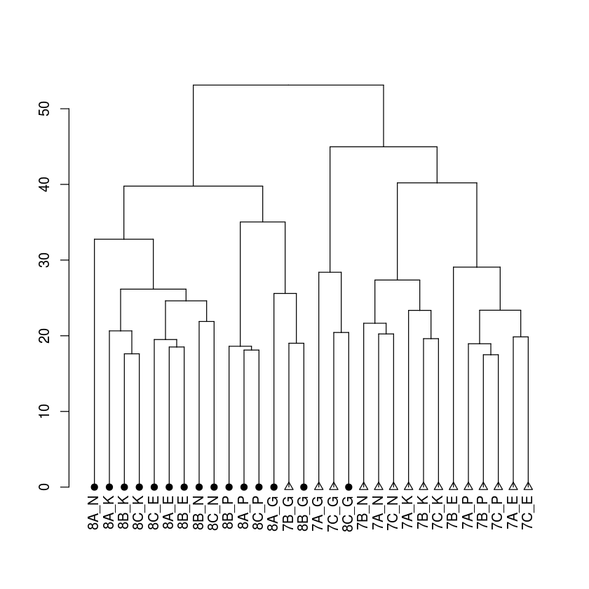
First add the treatment label. The symbol use for each leaf is controlled by “leaves_pch” (you can use label_cex and leaves_cex to control the relative size of the labels or leaves)

dend %>%
    set("labels_cex",1) %>%
    set("leaves_pch",trtlab) %>%
    set("leaves_cex",1) %>%
    plot

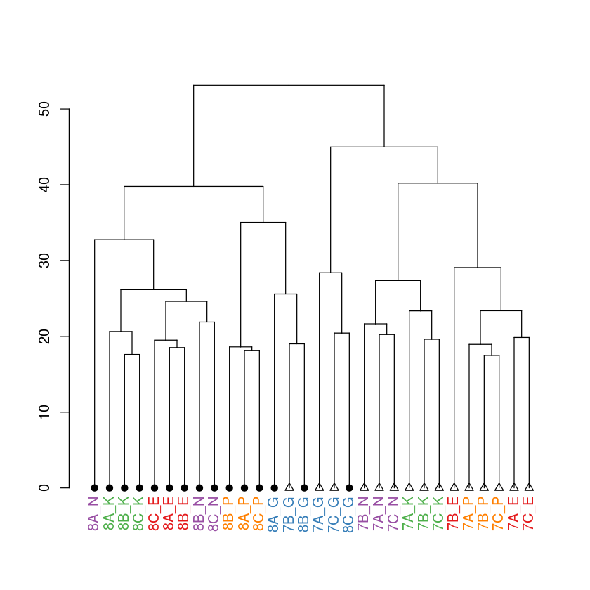
Now, lets add the group label to the above. The color of each label is controlled by “labels_col”

dend %>%
    set("labels_cex",1) %>%
    set("labels_col",grplab) %>%
    set("leaves_pch",trtlab) %>%
    set("leaves_cex",1) %>%
    plot

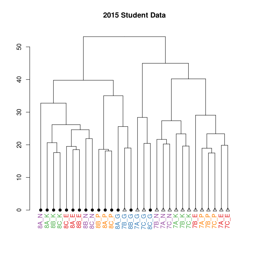
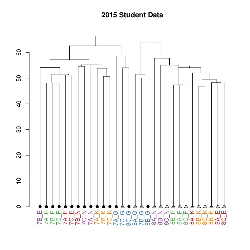
You can also add a title to the plot

dend %>%
    set("labels_cex",1) %>%
    set("labels_col",grplab) %>%
    set("leaves_pch",trtlab) %>%
    set("leaves_cex",1) %>%
    plot(main="2015 Student Data")

Repeat the analysis using expression data based on limma::voom with HC with single linkage:

Get expression matrix using voom

voomexp<-limma::voom(assay(dds))$E

Create dendrogram object based on single linkage

dend <- voomexp %>%
        t %>%
        dist %>%
        hclust(method="single") %>%
        as.dendrogram

Create plot

dend %>%
    set("labels_cex",1) %>%
    set("labels_col",grplab) %>%
    set("leaves_pch",trtlab) %>%
    set("leaves_cex",1) %>%
    plot(main="2015 Student Data")

Get Session Information

sessionInfo()

R version 3.3.1 (2016-06-21)
Platform: x86_64-pc-linux-gnu (64-bit)
Running under: Debian GNU/Linux 8 (jessie)

locale:
 [1] LC_CTYPE=en_US.UTF-8       LC_NUMERIC=C               LC_TIME=en_US.UTF-8
 [4] LC_COLLATE=en_US.UTF-8     LC_MONETARY=en_US.UTF-8    LC_MESSAGES=en_US.UTF-8
 [7] LC_PAPER=en_US.UTF-8       LC_NAME=C                  LC_ADDRESS=C
[10] LC_TELEPHONE=C             LC_MEASUREMENT=en_US.UTF-8 LC_IDENTIFICATION=C

attached base packages:
 [1] tools     parallel  stats4    stats     graphics  grDevices utils     datasets  methods
[10] base

other attached packages:
 [1] RColorBrewer_1.1-2         dplyr_0.5.0                dendextend_1.5.2
 [4] DESeq2_1.14.1              SummarizedExperiment_1.4.0 Biobase_2.34.0
 [7] GenomicRanges_1.26.4       GenomeInfoDb_1.10.3        IRanges_2.8.2
[10] S4Vectors_0.12.2           BiocGenerics_0.20.0

loaded via a namespace (and not attached):
 [1] viridis_0.4.0        viridisLite_0.2.0    jsonlite_1.1         splines_3.3.1
 [5] Formula_1.2-2        assertthat_0.1       latticeExtra_0.6-28  robustbase_0.92-7
 [9] RSQLite_1.0.0        backports_1.1.0      lattice_0.20-34      limma_3.30.13
[13] uuid_0.1-2           digest_0.6.10        XVector_0.14.1       checkmate_1.8.3
[17] colorspace_1.3-1     htmltools_0.3.5      Matrix_1.2-7.1       plyr_1.8.4
[21] XML_3.98-1.9         genefilter_1.56.0    zlibbioc_1.20.0      mvtnorm_1.0-6
[25] xtable_1.8-2         scales_0.4.1         whisker_0.3-2        BiocParallel_1.8.2
[29] htmlTable_1.9        tibble_1.2           annotate_1.52.1      ggplot2_2.2.1
[33] repr_0.7             nnet_7.3-12          lazyeval_0.2.0       survival_2.41-3
[37] magrittr_1.5         crayon_1.3.1         mclust_5.3           memoise_1.0.0
[41] evaluate_0.10        MASS_7.3-45          class_7.3-14         foreign_0.8-67
[45] data.table_1.10.4    trimcluster_0.1-2    stringr_1.0.0        kernlab_0.9-25
[49] munsell_0.4.3        locfit_1.5-9.1       cluster_2.0.5        AnnotationDbi_1.36.2
[53] fpc_2.1-10           grid_3.3.1           RCurl_1.95-4.8       pbdZMQ_0.2-3
[57] IRkernel_0.7         htmlwidgets_0.9      bitops_1.0-6         base64enc_0.1-3
[61] gtable_0.2.0         flexmix_2.3-14       DBI_0.5-1            R6_2.2.0
[65] gridExtra_2.2.1      prabclus_2.2-6       knitr_1.15.1         Hmisc_4.0-3
[69] modeltools_0.2-21    stringi_1.1.2        IRdisplay_0.4.3      Rcpp_0.12.8
[73] geneplotter_1.52.0   rpart_4.1-10         acepack_1.4.1        DEoptimR_1.0-8
[77] diptest_0.75-7