Principles and risks
of forecasting (pdf)
Famous forecasting
quotes
How to move data around
Get to know your data
Inflation adjustment (deflation)
Seasonal adjustment
Stationarity and differencing
The logarithm transformation
Seasonal adjustment
Multiplicative adjustment
Additive adjustment
Acronyms: SA, NSA, SAAR
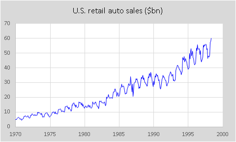
Multiplicative adjustment: Consider the graph of U.S. total retail sales of automobiles from January
1970 to May 1998, in units of billions of dollars, as reported at the time by
the U.S. Bureau of Economic Analysis:

Much of the trend is merely due to inflation. The values can be deflated, i.e.,
converted to units of constant rather than nominal dollars, by dividing them by
a suitable price index scaled to a value of 1.0 in whatever year is desired as
the base year. Here’s the
result of dividing by the U.S. consumer price index (CPI) scaled to 1.0 in
1990, which converts the units to billions of 1990 dollars:

(The data
can be found in this Excel file, and it is
also analyzed in further detail in the pages on seasonal ARIMA models on this
site.) There is still a general
upward trend, and the increasing amplitude of seasonal variations is suggestive
of a multiplicative seasonal pattern: the seasonal effect expresses
itself in percentage terms, so the absolute magnitude of the seasonal variations
increases as the series grows over time. Such a pattern can be removed by multiplicative
seasonal adjustment, which is accomplished by dividing each value of
the time series by a seasonal index (a number in the vicinity of 1.0) that
represents the percentage of normal typically observed in that season.
For example,
if December's sales are typically 130% of the normal monthly value (based on
historical data), then each December's sales would be seasonally adjusted by
dividing by 1.3. Similarly, if January's sales are typically only 90% of
normal, then each January's sales would be seasonally adjusted by dividing by
0.9. Thus, December's value would be adjusted downward while January's would be
adjusted upward, correcting for the anticipated seasonal effect. Depending on
how they were estimated from the data, the seasonal indices might remain the
same from one year to the next, or they might vary slowly with time.
The seasonal
indices computed by the Seasonal Decomposition procedure in Statgraphics are
constant over time, and are computed via the so-called "ratio-to-moving
average method." (For an explanation of this method, see the slides
on forecasting with seasonal adjustment and the notes on spreadsheet implementation of seasonal adjustment.)
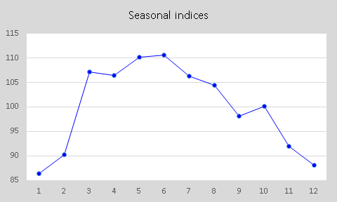
Here are the multiplicative seasonal indices for auto sales as computed by the
Seasonal Decomposition procedure in Statgraphics:

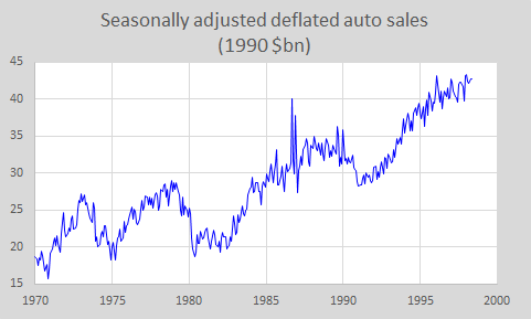
Finally,
here is the seasonally adjusted version of deflated auto sales that is obtained by
dividing each month's value by its estimated seasonal index:

Notice that
the pronounced seasonal pattern is gone, and what remains are the trend and
cyclical components of the data, plus random noise.
Additive
adjustment: As
an alternative to multiplicative seasonal adjustment, it is also possible to
perform additive seasonal adjustment. A time series whose seasonal
variations are roughly constant in magnitude, independent of the current
average level of the series, would be a candidate for additive seasonal
adjustment. In additive seasonal adjustment, each value of a time series is
adjusted by adding or subtracting a quantity that represents the
absolute amount by which the value in that season of the year tends to be below
or above normal, as estimated from past data.
Additive
seasonal patterns are somewhat rare in nature, but a series that has a natural
multiplicative seasonal pattern is converted to one with an additive seasonal
pattern by applying a logarithm transformation to the
original data. Therefore, if you are using seasonal adjustment in conjunction
with a logarithm transformation, you probably should use additive rather than
multiplicative seasonal adjustment. (In the Seasonal Decomposition and
Forecasting procedures in Statgraphics, you are given a choice between additive
and multiplicative seasonal adjustment.) (Return to top of
page.)
Acronyms: When examining the
descriptions of time series in Datadisk and other sources, the acronym SA
stands for "seasonally adjusted, whereas NSA stands for "not
seasonally adjusted. A seasonally adjusted annual rate (SAAR) is
a time series in which each period's value has been adjusted for seasonality
and then multiplied by the number of periods in a year, as though the same
value had been obtained in every period for a whole year. (Return
to top of page.)
Go on to next topic: Stationarity and differencing
