 ARIMA models for time series forecasting
Notes
on nonseasonal ARIMA models (pdf file)
Slides on seasonal and
nonseasonal ARIMA models (pdf file)
Introduction
to ARIMA: nonseasonal models
Identifying the order of differencing in an ARIMA model
Identifying the numbers of AR or MA terms in an ARIMA
model
Estimation of ARIMA models
Seasonal
differencing in ARIMA models
Seasonal random walk: ARIMA(0,0,0)x(0,1,0)
Seasonal random trend: ARIMA(0,1,0)x(0,1,0)
General seasonal models: ARIMA (0,1,1)x(0,1,1) etc.
Summary of rules for identifying ARIMA models
ARIMA models with regressors
The
mathematical structure of ARIMA models (pdf file)
Seasonal differencing
in ARIMA models
Seasonal difference (season-to-season change)
First difference
of seasonal difference
Data files:
Excel file with auto sales data
Statgraphics data and
model files (zip)
The
seasonal difference of a time series is the series of changes from one season
to the next. For monthly data, in which there are 12 periods in a season, the
seasonal difference of Y at period t is Yt - Yt-12. If
the seasonal difference of Y is stationary white noise (independently and
identically distributed values with no autocorrelation), then Y is described by
a seasonal random walk model: each value is a random
step away from the value that occurred exactly one season ago.
Seasonal
differencing is a crude form of additive seasonal adjustment: the "index"
which is subtracted from each value of the time series is simply the value that
was observed in the same season one year earlier. Seasonal differencing
therefore usually removes the gross features of seasonality from a series, as
well as most of the trend.
Seasonal
differencing and other aspects of seasonal ARIMA modeling to be discussed later
will be illustrated by the U.S. retail auto sales data, deflated to units of
1990 dollars, that was introduced on the seasonal adjustment page. Here
is a plot of that series, which is called "AUTOSALE/CPI" in the Statgraphics
file, for the period from January 1970 to May 1994:

Here is a
plot of the seasonal difference. Notice that little remains of the original
seasonal pattern or trend, although it now looks a bit like a random walk
rather than pure noise.
First
difference of seasonal difference: In the preceding two graphs, we see that the
first difference of AUTOSALE/CPI is far from random (it is still strongly
seasonal), and the seasonal difference is far from stationary (it resembles a
random walk). In this case, it appears that both kinds of differencing
are needed to render the series stationary and to account for the gross pattern
of seasonality. The first difference of the seasonal difference of a
monthly time series Y at period t is equal to (Yt - Yt-12)
- (Yt-1 - Yt-13). Equivalently, it is equal to (Yt
- Yt-1) - (Yt-12 - Yt-13). This is the amount
by which the change from the previous period to the current period is different
from the change that was observed exactly one year earlier. Thus, for example,
the first difference of the seasonal difference in September 1995 is equal to
the August-to-September change in 1995 minus the August-to-September change in
1994. If the first difference of the seasonal difference of Y is pure noise,
then Y is described by a seasonal random trend
model.
Here is a
plot of the first difference of the seasonal difference of AUTOSALE/CPI. Note
that it now appears stationary without obvious signs of seasonality. (We should
look at an autocorrelation plot to be sure that no seasonal pattern remains,
but at least the gross seasonal pattern has been eliminated.)
Go on to next topic: seasonal
random walk model
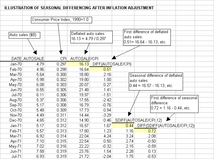
The
following spreadsheet shows how the seasonal difference and first difference of
the seasonal difference are calculated in this example:


