 ARIMA models for time
series forecasting
ARIMA models for time
series forecasting
Notes
on nonseasonal ARIMA models (pdf file)
Slides on seasonal and
nonseasonal ARIMA models (pdf file)
Introduction
to ARIMA: nonseasonal models
Identifying the order of differencing in an ARIMA model
Identifying the numbers of AR or MA terms in an ARIMA
model
Estimation of ARIMA models
Seasonal differencing in ARIMA models
Seasonal random walk: ARIMA(0,0,0)x(0,1,0)
Seasonal random trend: ARIMA(0,1,0)x(0,1,0)
General seasonal models: ARIMA (0,1,1)x(0,1,1) etc.
Summary of rules for identifying ARIMA models
ARIMA models with regressors
The
mathematical structure of ARIMA models (pdf file)
General seasonal ARIMA
models: (0,1,1)x(0,1,1) etc.
Outline of seasonal ARIMA modeling
Example: AUTOSALE series revisited
The often-used ARIMA(0,1,1)x(0,1,1) model: SRT model plus
MA(1) and SMA(1) terms
The ARIMA(1,0,0)x(0,1,0) model with constant: SRW model plus
AR(1) term
An improved version: ARIMA(1,0,1)x(0,1,1) with constant
Seasonal ARIMA versus exponential smoothing and seasonal
adjustment
What are the tradeoffs among the various seasonal models?
To log or not to log?
Data files:
Excel file with auto sales data
Statgraphics data and
model files (zip)
Outline
of seasonal ARIMA modeling:
- The
seasonal part of an ARIMA model has the same structure as the non-seasonal
part: it may have an AR factor, an MA factor, and/or an order of
differencing. In the seasonal part of the model, all of these factors
operate across multiples of lag s (the number of periods in a
season).
- A
seasonal ARIMA model is classified as an ARIMA(p,d,q)x(P,D,Q)
model, where P=number of seasonal autoregressive (SAR) terms, D=number of
seasonal differences, Q=number of seasonal moving average (SMA) terms
- In
identifying a seasonal model, the first step is to determine
whether or not a seasonal difference is needed, in addition to or
perhaps instead of a non-seasonal difference. You should look at time
series plots and ACF and PACF plots for all possible combinations of 0 or
1 non-seasonal difference and 0 or 1 seasonal difference. Caution:
don't EVER use more than ONE seasonal difference, nor more than TWO total
differences (seasonal and non-seasonal combined).
- If
the seasonal pattern is both strong and stable over time
(e.g., high in the Summer and low in the Winter, or vice versa), then you
probably should use a seasonal difference regardless of whether you
use a non-seasonal difference, since this will prevent the seasonal
pattern from "dying out" in the long-term forecasts. Let's add
this to our list of rules for identifying models
Rule 12: If the series has a strong and consistent seasonal pattern, then you should use an order of seasonal differencing--but never use more than one order of seasonal differencing or more than 2 orders of total differencing (seasonal+nonseasonal).
- The
signature of pure SAR or pure SMA behavior is similar to the
signature of pure AR or pure MA behavior, except that the pattern appears
across multiples of lag s in the ACF and PACF.
- For
example, a pure SAR(1) process has spikes in the ACF at lags s, 2s, 3s,
etc., while the PACF cuts off after lag s.
- Conversely,
a pure SMA(1) process has spikes in the PACF at lags s, 2s, 3s, etc.,
while the ACF cuts off after lag s.
- An
SAR signature usually occurs when the autocorrelation at the seasonal
period is positive, whereas an SMA signature usually occurs when
the seasonal autocorrelation is negative, hence:
Rule 13: If the autocorrelation at the seasonal period is positive, consider adding an SAR term to the model. If the autocorrelation at the seasonal period is negative, consider adding an SMA term to the model. Try to avoid mixing SAR and SMA terms in the same model, and avoid using more than one of either kind.
- Usually
an SAR(1) or SMA(1) term is sufficient. You will rarely encounter a
genuine SAR(2) or SMA(2) process, and even more rarely have enough data to
estimate 2 or more seasonal coefficients without the estimation algorithm
getting into a "feedback loop."
- Although
a seasonal ARIMA model seems to have only a few parameters, remember that
backforecasting requires the estimation of one or two seasons' worth of
implicit parameters to initialize it. Therefore, you should have at least
4 or 5 seasons of data to fit a seasonal ARIMA model.
- Probably
the most commonly used seasonal ARIMA model is the (0,1,1)x(0,1,1)
model--i.e., an MA(1)xSMA(1) model with both a seasonal and a non-seasonal
difference. This is essentially a "seasonal exponential
smoothing" model.
- When
seasonal ARIMA models are fitted to logged data, they are capable
of tracking a multiplicative seasonal pattern.
Example:
AUTOSALE series revisited
Recall that we
previously forecast the retail auto sales series by using
a combination of deflation, seasonal adjustment and exponential smoothing. Let's now try fitting the same series with
seasonal ARIMA models, using the same sample of data from January 1970 to May
1993 (281 observations). As before we will work with deflated auto
sales--i.e., we will use the series AUTOSALE/CPI as the input variable. Here
are the time series plot and ACF and PACF plots of the original series, which
are obtained in the Forecasting procedure by plotting the "residuals"
of an ARIMA(0,0,0)x(0,0,0) model with constant:


The
"suspension bridge" pattern in the ACF is typical of a series that is
both nonstationary and strongly seasonal. Clearly we need at least one order of
differencing. If we take a nonseasonal difference, the corresponding plots are
as follows:


The
differenced series (the residuals of a random-walk-with-growth model) looks
more-or-less stationary, but there is still very strong autocorrelation at the
seasonal period (lag 12).
Because the
seasonal pattern is strong and stable, we know (from Rule 12) that we will want
to use an order of seasonal differencing in the model. Here is what the
picture looks like after a seasonal difference (only):


The
seasonally differenced series shows a very strong pattern of positive
autocorrelation, as we recall from our earlier attempt to fit a seasonal random walk model. This could be an "AR
signature"--or it could signal the need for another difference.
If we take
both a seasonal and nonseasonal difference, following results are obtained:


These are,
of course, the residuals from the seasonal random trend
model that we fitted to the auto sales data earlier. We now see the
telltale signs of mild overdifferencing: the positive spikes in the ACF
and PACF have become negative.
What is the
correct order of differencing? One more piece of information that might be
helpful is a calculation of the error statistics of the series at each
level of differencing. We can compute
these by fitting the corresponding ARIMA models in which only differencing is
used:
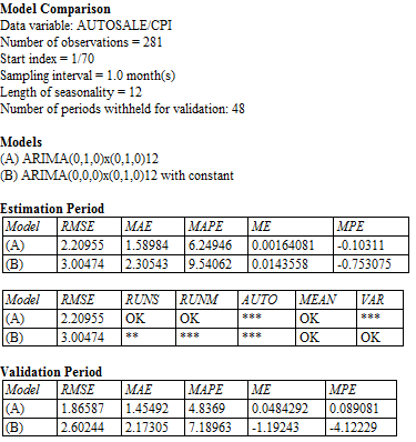
The smallest errors,
in both the estimation period and validation period, are obtained by model A,
which uses one difference of each type. This, together with the appearance of
the plots above, strongly suggests that we should use both a seasonal and a
nonseasonal difference. Note that, except for the gratuitious constant term,
model A is the seasonal random trend (SRT) model, whereas model B is just the
seasonal random walk (SRW) model. As we noted earlier when comparing these
models, the SRT model appears to fit better than the SRW model. In the analysis
that follows, we will try to improve these models through the addition of
seasonal ARIMA terms. Return to top of page.
The
often-used ARIMA(0,1,1)x(0,1,1) model: SRT model plus MA(1) and SMA(1) terms
Returning to the last
set of plots above, notice that with one
difference of each type there is a negative spike in the ACF at lag 1 and also
a negative spike in the ACF at lag 12, whereas the PACF shows a more
gradual "decay" pattern in the vicinity of both these lags. By
applying our rules for identifying ARIMA models
(specifically, Rule 7 and Rule 13), we may now conclude that the SRT model
would be improved by the addition of an MA(1) term and also an SMA(1) term.
Also, by Rule 5, we exclude the constant since two orders of
differencing are involved. If we do all this, we obtain the ARIMA(0,1,1)x(0,1,1) model, which is the most commonly used seasonal ARIMA model. Its forecasting equation is:
Ŷt =
Yt-12 + Yt-1 – Yt-13 - θ1et-1 – Θ1et-12 + θ1Θ1et-13
where θ1 is the MA(1)
coefficient and Θ1 (capital
theta-1) is the SMA(1) coefficient. Notice that this is just the seasonal
random trend model fancied-up by adding multiples of the errors at lags 1, 12,
and 13. Also, notice that the coefficient of the lag-13 error is the product of
the MA(1) and SMA(1) coefficients. This
model is conceptually similar to the Winters model insofar as it effectively
applies exponential smoothing to level, trend, and seasonality all at once,
although it rests on more solid theoretical foundations, particularly with
regard to calculating confidence intervals for long-term forecasts.
Its residual plots in
this case are as follows:


Although a slight amount of autocorrelation remains at lag 12, the overall appearance of the plots is good. The model fitting results show that the estimated MA(1) and SMA(1) coefficients (obtained after 7 iterations) are indeed significant:

The forecasts from
the model resemble those of the seasonal random trend model--i.e., they pick up
the seasonal pattern and the local trend at the end of the series--but they are
slightly smoother in appearance since both the seasonal pattern and the trend
are effectively being averaged (in a exponential-smoothing kind of way) over
the last few seasons:

What is this model really doing? You can think of it in the following
way. First it computes the difference
between each month’s value and an “exponentially weighted historical
average” for that month that is computed by applying exponential
smoothing to values that were observed in the same month in previous years, where
the amount of smoothing is determined by the SMA(1) coefficient. Then it applies simple exponential
smoothing to these differences in order to predict the deviation from the
historical average that will be observed next month. The value of the SMA(1) coefficient near
1.0 suggests that many seasons of data are being used to calculate the historical
average for a given month of the year. Recall that an MA(1) coefficient in an
ARIMA(0,1,1) model corresponds to 1-minus-alpha in the corresponding
exponential smoothing model, and that the average age of the data in an
exponential smoothing model forecast is 1/alpha. The SMA(1) coefficient has a
similar interpretation with respect to averages across seasons. Here its value of 0.91 suggests that the
average age of the data used for estimating the historical seasonal pattern is a
little more than 10 years (nearly half the length of the data set), which means
that an almost constant seasonal pattern is being assumed. The much smaller value of 0.5 for the
MA(1) coefficient suggests that relatively little smoothing is being done to
estimate the current deviation from the historical average for the same month,
so next month’s predicted deviation from its historical average will be
close to the deviations from the historical average that were observed over the
last few months.
The
ARIMA(1,0,0)x(0,1,0) model with constant: SRW model plus AR(1) term
The previous model
was a Seasonal Random Trend (SRT) model fine-tuned by the addition of MA(1) and
SMA(1) coefficients. An alternative ARIMA model for this series can be obtained
by substituting an AR(1) term for the nonseasonal difference--i.e., by adding
an AR(1) term to the Seasonal Random Walk (SRW) model. This will allow us to
preserve the seasonal pattern in the model while lowering the total amount of
differencing, thereby increasing the stability of the trend projections if
desired. (Recall that with one seasonal difference alone, the series did show a
strong AR(1) signature.) If we do this, we obtain an ARIMA(1,0,0)x(0,1,0) model
with constant, which yields the following results:

The AR(1) coefficient
is indeed highly significant, and the RMSE is only 2.06, compared to 3.00 for
the SRW model (Model B in the comparison report above). The forecasting
equation for this model is:
Ŷt =
μ + Yt-12 + ϕ1(Yt-1 - Yt-13)
The additional term
on the right-hand-side is a multiple of the seasonal difference observed in the
last month, which has the effect of correcting the forecast for the effect of
an unusually good or bad year. Here ϕ1 denotes the AR(1)
coefficient, whose estimated value is 0.73. Thus, for example, if sales last
month were X dollars ahead of sales one year earlier, then the quantity 0.73X
would be added to the forecast for this month. μ denotes
the CONSTANT in the forecasting
equation, whose estimated value is 0.20.
The estimated MEAN, whose value is 0.75, is the mean value of the
seasonally differenced series, which is the annual trend in the long-term
forecasts of this model. The
constant is (by definition) equal to the mean times 1 minus the AR(1)
coefficient: 0.2 = 0.75*(1 –
0.73).
The forecast plot
shows that the model indeed does a better job than the SRW model of tracking
cyclical changes (i.e., unusually good or bad years):

However, the MSE for
this model is still significantly larger than what we obtained for the
ARIMA(0,1,1)x(0,1,1) model. If we look at the plots of residuals, we see room
for improvement. The residuals still show some sign of cyclical variation:

The ACF and PACF suggest
the need for both MA(1) and SMA(1) coefficients:


An
improved version: ARIMA(1,0,1)x(0,1,1) with constant
If we add the
indicated MA(1) and SMA(1) terms to the preceding model, we obtain an ARIMA(1,0,1)x(0,1,1)
model with constant, whose forecasting equation is
Ŷt =
μ + Yt-12 + ϕ1(Yt-1 – Yt-13) - θ1et-1 – Θ1et-12 + θ1Θ1et-13
This is nearly the same as the ARIMA(0,1,1)x(0,1,1) model
except that it replaces the nonseasonal difference with an AR(1) term (a
"partial difference") and it incorporates a constant term
representing the long-term trend.
Hence,
this model assumes a more stable trend than the ARIMA(0,1,1)x(0,1,1) model, and
that is the principal difference between them.
The model-fitting results are as follows:

Notice that the
estimated AR(1) coefficient (ϕ1 in the model equation) is 0.96, which
is very close to 1.0 but not so close as to suggest that it absolutely ought to
be replaced with a first difference:
its standard error is 0.02, so it is about 2 standard errors from
1.0. The other statistics of the
model (the estimated MA(1) and SMA(1) coefficients and error statistics in the
estimation and validation periods) are otherwise nearly identical to those of
the ARIMA(0,1,1)x(0,1,1) model. (The estimated MA(1) and SMA(1) coefficients
are 0.45 and 0.91 in this model vs. 0.48 and 0.91 in the other.)
The estimated MEAN of
0.68 is the predicted long-term trend (average annual increase). This is essentially the same value that was
obtained in the (1,0,0)x(0,1,0)-with-constant model. The standard error of the
estimated mean is 0.26, so the difference between 0.75 and 0.68 is not
significant.
If the constant was not included in this model, it would
be a damped-trend model: the trend
in its very-long-term forecasts would gradually flatten out.
The point forecasts
from this model look quite similar to those of the (0,1,1)x(0,1,1) model,
because the average trend is similar to the local trend at the end of the
series. However, the confidence intervals for this model widen somewhat less
rapidly because of its assumption that the trend is stable. Notice that the
confidence limits for the two-year-ahead forecasts now stay within the
horizontal grid lines at 24 and 44, whereas those of the (0,1,1)x(0,1,1) model
did not:

Seasonal
ARIMA versus exponential smoothing and seasonal adjustment: Now let's compare the
performance the two best ARIMA models against simple and linear exponential
smoothing models accompanied by multiplicative seasonal adjustment, and the
Winters model, as shown in the slides
on forecasting with seasonal adjustment:

The error statistics
for the one-period-ahead forecasts for all the models are extremely close in
this case. It is hard to pick a
“winner” based on these numbers alone. Return to top of page.
What
are the tradeoffs among the various seasonal models? The three models that
use multiplicative seasonal adjustment deal with seasonality in an explicit
fashion--i.e., seasonal indices are broken out as an explicit part of the
model. The ARIMA models deal with
seasonality in a more implicit manner--we can't easily see in the ARIMA output
how the average December, say, differs from the average July. Depending on
whether it is deemed important to isolate the seasonal pattern, this might be a
factor in choosing among models. The ARIMA models have the advantage that, once
they have been initialized, they have fewer "moving parts" than the
exponential smoothing and adjustment models and as such they may be less likely
to overfit the data. ARIMA models
also have a more solid underlying theory with respect to the calculation of
confidence intervals for longer-horizon forecasts than do the other models.
There are more
dramatic differences among the models with respect to the behavior of their
forecasts and confidence intervals for forecasts more than 1 period into the
future. This is where the
assumptions that are made with
respect to changes in the trend and seasonal pattern are very important.
Between the two ARIMA
models, one (model A) estimates a time-varying trend, while the other (model B)
incorporates a long-term average trend. (We could, if we desired, flatten out
the long-term trend in model B by suppressing the constant term.) Among the
exponential-smoothing-plus-adjustment models, one (model C) assumes a flat
trend, while the other (model D) assumes a time-varying trend. The Winters model (E) also assumes a
time-varying trend.
Models that assume a
constant trend are relatively more confident in their long-term forecasts than
models that do not, and this will usually be reflected in the extent to which
confidence intervals for forecasts get wider at longer forecast horizons. Models that do not assume time-varying
trends generally have narrower confidence intervals for longer-horizon
forecasts, but narrower is not better unless this assumption is correct.
The two exponential
smoothing models combined with seasonal adjustment assume that the seasonal
pattern has remained constant over the 23 years in the data sample, while the
other three models do not. Insofar
as the seasonal pattern accounts for most of the month-to-month variation in
the data, getting it right is important for forecasting what will happen
several months into the future. If
the seasonal pattern is believed to have changed slowly over time, another
approach would be to just use a shorter data history for fitting the models
that estimate fixed seasonal indices.
For the record, here
are the forecasts and 95% confidence limits for May 1995 (24 months ahead)
that are produced by the five
models:
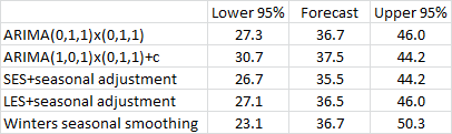

The point forecasts
are actually surprisingly close to each other, relative to the widths of all
the confidence intervals. The SES point forecast is the lowest, because it is
the only model that does not assume an upward trend at the end of the
series. The ARIMA
(1,0,1)x(0,1,1)+c model has the narrowest confidence limits, because it assumes
less time-variation in the parameters than the other models. Also, its point
forecast is slightly larger than those of the other models, because it is
extrapolating a long-term trend rather than a short-term trend (or zero
trend).
The Winters model is
the least stable of the models and its forecast therefore has the widest
confidence limits, as was apparent in the detailed forecast plots for the
models. And the forecasts and
confidence limits of the ARIMA(0,1,1)x(0,1,1) model and those of the
LES+seasonal adjustment model are virtually identical!
To
log or not to log? Something
that we have not yet done, but might have, is include a log transformation as
part of the model. Seasonal ARIMA models are inherently additive models,
so if we want to capture a multiplicative seasonal pattern, we must do
so by logging the data prior to fitting the ARIMA model. (In Statgraphics, we
would just have to specify "Natural Log" as a modeling option--no big
deal.) In this case, the deflation transformation seems to have done a
satisfactory job of stabilizing the amplitudes of the seasonal cycles, so there
does not appear to be a compelling reason to add a log transformation as far as
long term trends are concerned. If the residuals showed a marked increase in
variance over time, we might decide otherwise.
There is still a
question of whether the errors of these models have a consistent variance across months of the year. If they don’t, then confidence
intervals for forecasts might tend to be too wide or too narrow according to
the season. The residual-vs-time
plots do not show an obvious problem in this regard, but to be thorough, it
would be good to look at the error variance by month. If there is indeed a problem, a log
transformation might fix it. Return to top of page.
Go on to next topic: summary of rules for identifying ARIMA models