Linear trend model

If the variable of interest is a time series, then naturally it is important to identify and fit any systematic time patterns which may be present. Consider again the variable X1 that was analyzed on the page for the mean model, and suppose that it is a time series. Its graph looks like this:

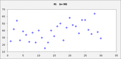
(The file containing this data and the models below can be found here.) There is indeed a suggestion of a time pattern, namely that the local mean value appears somewhat higher at the end of the series than at the beginning. There are several ways in which a change in the mean over time could be modeled. Possibly it underwent a “step change” at some point. In fact, the sample mean of the first 15 values of X1 is 32.3 with a standard error of 2.6, and the sample mean of the last 15 values is 44.7 with a standard error of 2.8. If 95% confidence intervals for these two means are calculated (approximately) by adding or subtracting two standard errors, the intervals do not overlap, so the difference in means is statistically very significant. If there is independent evidence for a sudden change in the mean in the middle of the sample, then it might make sense to break up the data into subsets or else fit a regression model with a dummy variable whose value is equal to zero up the point at which the change occurred and equal to 1 afterward. The estimated coefficient of such a variable would measure the magnitude of the change.

Another possibility is that the local mean is increasing gradually over time, i.e., that there is a constant trend. If that is the case, then it might be appropriate to fit a sloping line rather than a horizontal line to the entire series. This is a linear trend model, also known as a trend-line model. It is a special case of a simple regression model in which the independent variable is just a time index variable, i.e., 1, 2, 3, ... or some other equally spaced sequence of numbers. When it is estimated by regression, the trend line is the unique line that minimizes the sum of squared deviations from the data, measured in the vertical direction. (More information about this and other properties of regression models is provided in the regression pages on this web site.)

If you are plotting the data in Excel, you can just right-click on the graph and select "Add Trendline" from the pop-up menu to slap a trend line on it. You can also use the trendline options to display R-squared and the estimated slope and intercept, but no other numerical output, as shown here:

The intercept of the trend line (the point at which the line crosses the y-axis) is 30.5 and its slope (the increase per period) is 0.516. More detail can be obtained by fitting the regression model using statistical software such as RegressIt. Here is some of the standard output that is provided by RegressIt, including 50% confidence bands around the regression line:

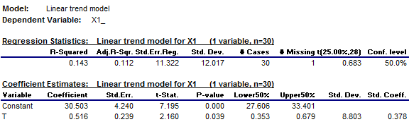
(The time index variable was named T in this data set.) R-squared for this model is 0.143, which means that the variance of the regression model's errors is 14.3% less than the variance of the mean model's errors, i.e., the model has “explained” 14.3% of the variance in X1. Adjusted R-squared, which is 0.112, is the fraction by which the square of the standard error of the regression is less than the variance of the mean model's errors, and it is an unbiased measure of the fraction of variance that has been explained. (See this page for a more thorough discussion of R-squared and adjusted R-squared.)

So, the linear trend model does improve a bit on the mean model for this time series. Is the improvement statistically significant? To help answer that question, we can look at the t-statistic of the slope coefficient, whose value is 2.16, and its associated P-value, which is 0.039. These statistics indicate that the estimated slope is different from zero at (better than) the 0.05 level of significance, so the model passes that conventional test, but not by a lot.

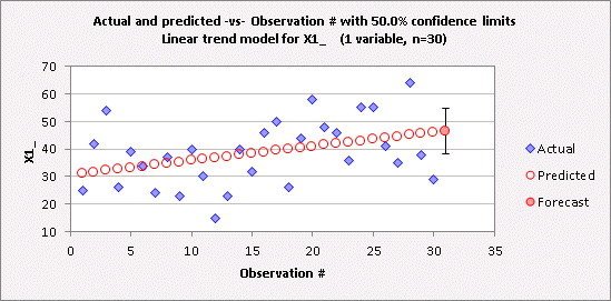
If the objective of the analysis is to forecast what will happen next, the most important issue in comparing the models is the extent to which they make different predictions. Here is a table and chart of the forecast that the linear trend model produces for X1 in period 31, with 50% confidence limits:

And here is the corresponding forecast produced by the mean model:

Notice that the mean model’s point forecast for period 31 (38.5) is almost the same as the lower 50% limit (38.2) for the linear trend model’s forecast. Roughly speaking, the mean model predicts that there is a 50% chance of observing a value less than 38.5 in period 31, while the linear trend model predicts that there is only a 25% chance of this happening.

Which model should be chosen? The data argues in favor of the linear trend model, although consideration should also be given to the question of whether it is logical to assume that this series has a steady upward trend (as opposed, say, to no trend or a randomly changing trend), based on everything else that is known about it. The trend that has been estimated from this sample of data is statistically significant but not overwhelmingly so.

Here is a graph of another variable, X2, which exhibits a much stronger upward trend:

If a linear trend model is fitted, the following results are obtained, with 95% confidence limits shown:

R-squared is 92% for this model! That means it is very good, right? Well, no. The straight line does not actually do a very good job of capturing the fine detail in the time pattern. Here is a plot of the errors (“residuals”) of the model versus time:

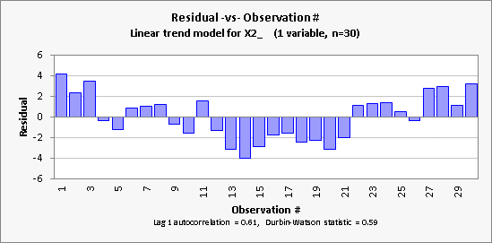
It is seen here (and was also evident on the regression line plot, if you look closely) that the linear trend model for X2 has a tendency to make an error of the same sign for many periods in a row. This tendency is measured in statistical terms by the lag-1 autocorrelation and Durbin-Watson statistic. If there is no time pattern, the lag-1 autocorrelation should be very close to zero, and the Durbin-Watson statistic ought to be very close to 2, which is not the case here. If the model has succeeded in extracting all the "signal" from the data, there should be no pattern at all in the errors: the error in the next period should not be correlated with any previous errors. The linear trend model obviously fails the autocorrelation test in this case.

If we are interested in using the model to predict the future, the fact that 8 out its last 9 errors have been positive and they appear to be getting worse is cause for concern. Here is a chart of the predictions, together with the forecast and 95% confidence interval for period 31. The forecast clearly appears to be too low, given what X2 has been doing lately and given that in the past it did not show a tendency to quickly return to the regression line after wandering away from it.

For this time series, a better model would be a random-walk-with-drift model, which merely predicts that the next period’s value will be the same as the current period’s value, plus a constant. The standard deviation of the errors made by the random-walk-with-drift model is simply the standard deviation of the period-to-period change (the so-called “first difference”) of the variable, which is 1.75 for X2. This is significantly less than the standard error of the regression for the linear trend model, which is 2.28. The random-walk-with-drift model would predict the value of X2 in period 31 to be slightly above its observed value in period 30, which seems more realistic here.

Although trend lines have their uses as visual aids, they are often poor for purposes of forecasting outside the historical range of the data. Most time series that arise in nature and economics do not behave as though there are straight lines fixed in space to which they want to return some day. Rather, their levels and trends undergo evolution. The linear trend model tries to find the slope and intercept that give the best average fit to all the past data, and unfortunately its deviation from the data is often greatest at the very end of the time series (the “business end” as I like to call it), where the forecasting action is! When trying to project an assumed linear trend into the future, we would like to know the current values of the slope and intercept--i.e., the values that will give the best fit to the next few periods' data. We will see that other forecasting models often do a better job of this than the simple linear trend model. (Return to top of page.)

For more discussion of the linear trend model, and its comparison to the mean model for another data sample, see pages 12-16 of the handout: “Review of basic statistics and the simplest forecasting model: the mean model.” For complete details of how the slope and intercept are estimated and how confidence limits for forecasts are computed, see the mathematics of simple regression page.

Go to next topic: random walk model.