Seasonal ARIMA models

Outline of seasonal ARIMA modeling
Example: AUTOSALE series revisited
The oft-used ARIMA(0,1,1)x(0,1,1) model: SRT model plus MA(1) and SMA(1) terms
The ARIMA(1,0,0)x(0,1,0) model with constant: SRW model plus AR(1) term
An improved version: ARIMA(1,0,1)x(0,1,1) with constant
Seasonal ARIMA versus exponential smoothing and seasonal adjustment
What are the tradeoffs among the various seasonal models?
To log or not to log?

Outline of seasonal ARIMA modeling:

The seasonal part of an ARIMA model has the same structure as the non-seasonal part: it may have an AR factor, an MA factor, and/or an order of differencing. In the seasonal part of the model, all of these factors operate across multiples of lag s (the number of periods in a season).
A seasonal ARIMA model is classified as an ARIMA(p,d,q)x(P,D,Q) model, where P=number of seasonal autoregressive (SAR) terms, D=number of seasonal differences, Q=number of seasonal moving average (SMA) terms
In identifying a seasonal model, the first step is to determine whether or not a seasonal difference is needed, in addition to or perhaps instead of a non-seasonal difference. You should look at time series plots and ACF and PACF plots for all possible combinations of 0 or 1 non-seasonal difference and 0 or 1 seasonal difference. Caution: don't EVER use more than ONE seasonal difference, nor more than TWO total differences (seasonal and non-seasonal combined).
If the seasonal pattern is both strong and stable over time (e.g., high in the Summer and low in the Winter, or vice versa), then you probably should use a seasonal difference regardless of whether you use a non-seasonal difference, since this will prevent the seasonal pattern from "dying out" in the long-term forecasts. Let's add this to our list of rules for identifying models

Rule 12: If the series has a strong and consistent seasonal pattern, then you should use an order of seasonal differencing--but never use more than one order of seasonal differencing or more than 2 orders of total differencing (seasonal+nonseasonal).
The signature of pure SAR or pure SMA behavior is similar to the signature of pure AR or pure MA behavior, except that the pattern appears across multiples of lag s in the ACF and PACF.
For example, a pure SAR(1) process has spikes in the ACF at lags s, 2s, 3s, etc., while the PACF cuts off after lag s.
Conversely, a pure SMA(1) process has spikes in the PACF at lags s, 2s, 3s, etc., while the ACF cuts off after lag s.
An SAR signature usually occurs when the autocorrelation at the seasonal period is positive, whereas an SMA signature usually occurs when the seasonal autocorrelation is negative, hence:

Rule 13: If the autocorrelation at the seasonal period is positive, consider adding an SAR term to the model. If the autocorrelation at the seasonal period is negative, consider adding an SMA term to the model. Do not mix SAR and SMA terms in the same model, and avoid using more than one of either kind.
Usually an SAR(1) or SMA(1) term is sufficient. You will rarely encounter a genuine SAR(2) or SMA(2) process, and even more rarely have enough data to estimate 2 or more seasonal coefficients without the estimation algorithm getting into a "feedback loop."
Although a seasonal ARIMA model seems to have only a few parameters, remember that backforecasting requires the estimation of one or two seasons' worth of implicit parameters to initialize it. Therefore, you should have at least 4 or 5 seasons of data to fit a seasonal ARIMA model.
Probably the most commonly used seasonal ARIMA model is the (0,1,1)x(0,1,1) model--i.e., an MA(1)xSMA(1) model with both a seasonal and a non-seasonal difference. This is essentially a "seasonal exponential smoothing" model.
When seasonal ARIMA models are fitted to logged data, they are capable of tracking a multiplicative seasonal pattern.

Example: AUTOSALE series revisited

Recall that we previously forecast the retail auto sales series by using a combination of deflation, seasonal adjustment and exponential smoothing. Let's now try fitting the same series with seasonal ARIMA models. As before we will work with deflated auto sales--i.e., we will use the series AUTOSALE/CPI as the input variable. Here are the time series plot and ACF and PACF plots of the original series, which are obtained in the Forecasting procedure by plotting the "residuals" of an ARIMA(0,0,0)x(0,0,0) model with constant:

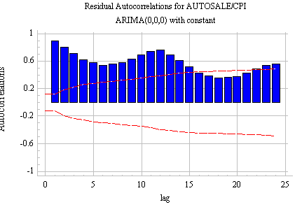
The "suspension bridge" pattern in the ACF is typical of a series that is both nonstationary and strongly seasonal. Clearly we need at least one order of differencing. If we take a nonseasonal difference, the corresponding plots are as follows:

The differenced series (the residuals of a random-walk-with-growth model) looks more-or-less stationary, but there is still very strong autocorrelation at the seasonal period (lag 12).

Because the seasonal pattern is strong and stable, we know (from Rule 12) that we will want to use an order of seasonal differencing in the model. Here is what the picture looks like after a seasonal difference (only):

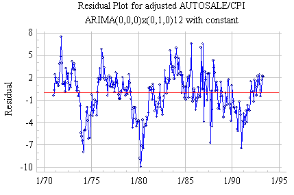
The seasonally differenced series shows a very strong pattern of positive autocorrelation, as we recall from our earlier attempt to fit a seasonal random walk model. This could be an "AR signature"--or it could signal the need for another difference.

If we take both a seasonal and nonseasonal difference, following results are obtained:

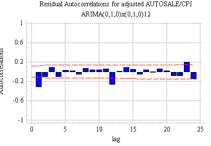
These are, of course, the residuals from the seasonal random trend model that we fitted to the auto sales data earlier. We now see the telltale signs of mild overdifferencing: the positive spikes in the ACF and PACF have become negative.

What is the correct order of differencing? One more piece of information that might be helpful is a calculation of the variance of the series at each level of differencing. This is just the MSE that results from fitting the various difference-only ARIMA models:

Model Comparison
----------------
Data variable: AUTOSALE/CPI
Number of observations = 281
Start index = 1/70            
Sampling interval = 1.0 month(s)
Length of seasonality = 12
Number of periods withheld for validation: 48

Models
------
(A) ARIMA(0,0,0) with constant
(B) ARIMA(0,1,0) with constant
(C) ARIMA(0,0,0)x(0,1,0)12 with constant
(D) ARIMA(0,1,0)x(0,1,0)12 with constant

Estimation Period
Model  MSE          MAE          MAPE         ME           MPE
------------------------------------------------------------------------
(A)    26.2264      4.16826      17.1422      -0.00725956  -4.18066     
(B)    5.67387      1.79003      7.13332      0.007303     -0.413321    
(C)    9.02848      2.30545      9.54065      0.0144368    -0.752748    
(D)    4.9044       1.59         6.25023      -0.00265268  -0.120404

We see that the lowest MSE is obtained by model D which uses one difference of each type. This, together with the appearance of the plots above, strongly suggests that we should use both a seasonal and a nonseasonal difference. Note that, except for the gratuitious constant term, model D is the seasonal random trend (SRT) model, whereas model B is just the seasonal random walk (SRW) model. As we noted earlier when comparing these models, the SRT model appears to fit better than the SRW model. In the analysis that follows, we will try to improve these models through the addition of seasonal ARIMA terms.

The oft-used ARIMA(0,1,1)x(0,1,1) model: SRT model plus MA(1) and SMA(1) terms

Returning to the last set of plots above, notice that with one difference of each type there is a negative spike in the ACF at lag 1 and also a negative spike in the ACF at lag 12, whereas the PACF shows a more gradual "decay" pattern in the vicinity of both these lags. By applying our rules for identifying ARIMA models (specifically, Rule 7 and Rule 13), we may now conclude that the SRT model would be improved by the addition of an MA(1) term and also an SMA(1) term. Also, by Rule 5, we exclude the constant since two orders of differencing are involved. If we do all this, we obtain the often-used ARIMA(0,1,1)x(0,1,1) model, whose residual plots are as follows:

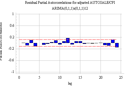
Although a slight amount of autocorrelation remains at lag 12, the overall appearance of the plots is good. The model fitting results show that the estimated MA(1) and SMA(1) coefficients (obtained after 7 iterations) are indeed significant:

Analysis Summary
Data variable: AUTOSALE/CPI
Number of observations = 281
Start index = 1/70            
Sampling interval = 1.0 month(s)
Length of seasonality = 12

Forecast Summary
----------------
Nonseasonal differencing of order: 1
Seasonal differencing of order: 1

Forecast model selected: ARIMA(0,1,1)x(0,1,1)12
Number of forecasts generated: 24
Number of periods withheld for validation: 48

            Estimation      Validation
Statistic   Period          Period
--------------------------------------------
MSE         2.77303         1.83711         
MAE         1.23574         1.05651         
MAPE        4.89559         3.47061         
ME          0.00985809      -0.135525       
MPE         -0.246026       -0.614371       

                            ARIMA Model Summary
Parameter           Estimate        Stnd. Error     t               P-value
----------------------------------------------------------------------------
MA(1)               0.479676        0.0591557       8.1087          0.000000
SMA(1)              0.906532        0.0267735       33.8593         0.000000
----------------------------------------------------------------------------
Backforecasting: yes
Estimated white noise variance = 2.85055 with 266 degrees of freedom
Estimated white noise standard deviation = 1.68836
Number of iterations: 7

The ARIMA(0,1,1)x(0,1,1) model is basically a Seasonal Random Trend (SRT) model fine-tuned by the addition of MA(1) and SMA(1) terms to correct for the mild overdifferencing that resulted from taking two total orders of differencing. THIS IS PROBABLY THE MOST COMMONLY USED SEASONAL ARIMA MODEL. The forecasts from the model resemble those of the seasonal random trend model--i.e., they pick up the seasonal pattern and the local trend at the end of the series--but they are slightly smoother in appearance since both the seasonal pattern and the trend are effectively being averaged (in a exponential-smoothing kind of way) over the last few seasons:

Indeed, the value of the SMA(1) coefficient near 1.0 suggests that many seasons of data are being averaged over to estimate the seasonal pattern. (Recall that an MA(1) coefficient corresponds to "1 minus alpha" in an exponential smoothing model, and that a large MA(1) coefficient therefore corresponds to a small alpha--i.e., a large average age of the data in the smoothed forecast. The SMA(1) coefficient similarly corresponds to "1 minus" a seasonal smoothing coefficient--and a large value of the SMA(1) coefficient suggests a large average age measured in units of seasons of data.) The smaller value of the MA(1) coefficient suggests that relatively little smoothing is being done to estimate the local level and trend--i.e., only the last few months of data are being used for that purpose.

The forecasting equation for this model is:

where little-theta is the MA(1) coefficient and big-theta is the SMA(1) coefficient. Notice that this is just the seasonal random trend model fancied-up by adding multiples of the errors at lags 1, 12, and 13. Also, notice that the coefficient of the lag-13 error is the product of the MA(1) and SMA(1) coefficients.

The ARIMA(1,0,0)x(0,1,0) with constant: SRW model plus AR(1) term

The previous model was a Seasonal Random Trend (SRT) model fine-tuned by the addition of MA(1) and SMA(1) coefficients. An alternative ARIMA model for this series can be obtained by substituting an AR(1) term for the nonseasonal difference--i.e., by adding an AR(1) term to the Seasonal Random Walk (SRW) model. This will allow us to preserve the seasonal pattern in the model while lowering the total amount of differencing, thereby increasing the stability of the trend projections if desired. (Recall that with one seasonal difference alone, the series did show a strong AR(1) signature.) If we do this, we obtain an ARIMA(1,0,0)x(0,1,0) model with constant, which yields the following results:

Analysis Summary
Data variable: AUTOSALE/CPI
Number of observations = 281
Start index = 1/70            
Sampling interval = 1,0 month(s)
Length of seasonality = 12

Forecast Summary
----------------
Seasonal differencing of order: 1
Forecast model selected: ARIMA(1,0,0)x(0,1,0)12 with constant
Number of forecasts generated: 24
Number of periods withheld for validation: 48

            Estimation      Validation
Statistic   Period          Period
--------------------------------------------
MSE         4,24175         3,04301         
MAE         1,4508          1,44661         
MAPE        5,73812         4,78971         
ME          0,0209967       -0,274249       
MPE         -0,214828       -1,00671        

                            ARIMA Model Summary
Parameter           Estimate        Stnd. Error     t               P-value
----------------------------------------------------------------------------
AR(1)               0,72972         0,046205        15,7931         0,000001
Mean                0,75596         0,508192        1,48755         0,138051
Constant            0,204321        
----------------------------------------------------------------------------
Backforecasting: yes
Estimated white noise variance = 4,24182 with 267 degrees of freedom
Estimated white noise standard deviation = 2,05957
Number of iterations: 1

The AR(1) coefficient is indeed highly significant, and the MSE is only 4.24, compared to the 9.028 for the unadulterated SRW model (Model B in the comparison report above). The forecasting equation for this model is:

The additional term on the right-hand-side is a multiple of the seasonal difference observed in the last month, which has the effect of correcting the forecast for the effect of an unusually "good" or "bad" year. Here "phi" denotes the AR(1) coefficient, whose estimated value is 0.73. Thus, for example, if sales last month were X dollars ahead of sales one year earlier, then the quantity 0.73X would be added to the forecast for this month.

The forecast plot shows that the model indeed does a better job than the SRW model of tracking cyclical changes (i.e., unusually good or bad years):

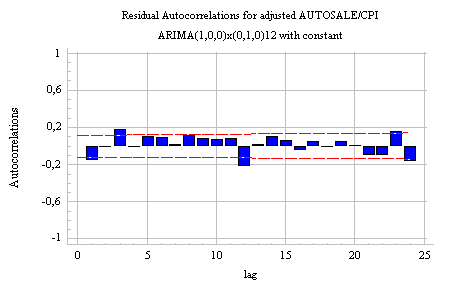
However, the MSE for this model is still significantly larger than what we obtained for the ARIMA(0,1,1)x(0,1,1) model. If we look at the plots of residuals, we see room for improvement. The residuals still show some sign of cyclical variation:

The ACF and PACF suggest the need for both MA(1) and SMA(1) coefficients:

An improved version: ARIMA(1,0,1)x(0,1,1) with constant

If we add the indicated MA(1) and SMA(1) terms to the preceding model, we obtain an ARIMA(1,0,1)x(0,1,1) model with constant. This is nearly the same as the ARIMA(0,1,1)x(0,1,1) model except that it replaces the nonseasonal difference with an AR(1) term (a "partial difference") and it incorporates a constant term representing the long-term trend. Hence, this model assumes a more stable long-term trend than the ARIMA(0,1,1)x(0,1,1) model. The model-fitting results are as follows:

Analysis Summary
Data variable: AUTOSALE/CPI
Number of observations = 281
Start index = 1/70            
Sampling interval = 1.0 month(s)
Length of seasonality = 12

Forecast Summary
----------------
Seasonal differencing of order: 1

Forecast model selected: ARIMA(1,0,1)x(0,1,1)12 with constant
Number of forecasts generated: 24
Number of periods withheld for validation: 48

            Estimation      Validation
Statistic   Period          Period
--------------------------------------------
MSE         2.75399         1.81308         
MAE         1.22287         1.05989         
MAPE        4.84797         3.49931         
ME          0.0297479       -0.262108       
MPE         -0.23536        -1.04485        

                            ARIMA Model Summary
Parameter           Estimate        Stnd. Error     t               P-value
----------------------------------------------------------------------------
AR(1)               0.959688        0.0220179       43.5868         0.000000
MA(1)               0.446023        0.0675235       6.60545         0.000000
SMA(1)              0.905846        0.0272139       33.2861         0.000000
Mean                0.681967        0.259388        2.62914         0.009060
Constant            0.0274918       
----------------------------------------------------------------------------
Backforecasting: yes
Estimated white noise variance = 2.80968 with 265 degrees of freedom
Estimated white noise standard deviation = 1.67621
Number of iterations: 9

Notice that the estimated AR(1) coefficient is very close to 1.0 (in fact, less than two standard errors away from 1.0) and that the other statistics of the model (the estimated MA(1) and SMA(1) coefficients and error statistics in the estimation and validation periods) are otherwise nearly identical to those of the previous model. A constant term has been included in this model because it has only one order of differencing, and the long-term forecasts from the model will therefore reflect the average trend over the whole history of the series rather than the local trend at the end of the series--this is the principal difference between this model and the preceding one. The estimated MEAN of 0.68 is the average annual increase.

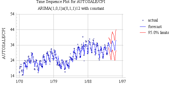
The forecasts from this model look quite similar to those of the preceding model, because the average trend is similar to the local trend at the end of the series. However, the confidence intervals for the model with a lower order of total differencing widen somewhat less rapidly. Notice that the confidence limits for the two-year-ahead forecasts now stay within the horizontal grid lines at 24 and 44:

The forecasting equation for this model is:

This is the same as the equation for the ARIMA(0,1,1)x(0,1,1) model, except that an AR(1) coefficient ("phi") now multiplies the Y(t-1)-Y(t-13) term, and a CONSTANT (mu) has been added. When phi is equal to 1 and mu is equal to zero, it becomes exactly the same as the previous equation--i.e., the AR(1) term becomes equivalent to a nonseasonal difference.

Seasonal ARIMA versus exponential smoothing and seasonal adjustment: Now let's compare the performance the ARIMA models against simple and linear exponential smoothing models accompanied by multiplicative seasonal adjustment:

Model Comparison
----------------
Data variable: AUTOSALE/CPI
Number of observations = 281
Start index = 1/70            
Sampling interval = 1.0 month(s)
Length of seasonality = 12
Number of periods withheld for validation: 48

Models
------
(A) ARIMA(0,1,0)x(0,1,0)12
(B) ARIMA(0,1,1)x(0,1,1)12
(C) ARIMA(1,0,1)x(0,1,1)12 with constant
(D) Simple exponential smoothing with alpha = 0.4772
    Seasonal adjustment: Multiplicative
(E) Brown's linear exp. smoothing with alpha = 0.2106
    Seasonal adjustment: Multiplicative

Estimation Period
Model  MSE          MAE          MAPE         ME           MPE
------------------------------------------------------------------------
(A)    4.8821       1.58984      6.24946      0.00164081   -0.10311     
(B)    2.77303      1.23574      4.89559      0.00985809   -0.246026    
(C)    2.75399      1.22287      4.84797      0.0297479    -0.23536     
(D)    2.639        1.18753      4.76707      0.131989     0.233418     
(E)    2.78296      1.24417      5.03819      0.00321996   -0.146439    

Model  RMSE         RUNS  RUNM  AUTO  MEAN  VAR
-----------------------------------------------
(A)    2.20955       OK    *     ***   OK   ***  
(B)    1.66524       OK    OK    OK    OK   ***  
(C)    1.65951       OK    OK    *     OK   ***  
(D)    1.6245        OK    OK    ***   OK   ***  
(E)    1.66822       OK    OK    ***   OK   ***  

Validation Period
Model  MSE          MAE          MAPE         ME           MPE
------------------------------------------------------------------------
(A)    3.4813       1.45537      4.83928      0.0460732    0.0818369    
(B)    1.83711      1.05651      3.47061      -0.135525    -0.614371    
(C)    1.81308      1.05989      3.49931      -0.262108    -1.04485     
(D)    1.87575      1.07203      3.48819      -0.040363    -0.279181    
(E)    1.908        1.07484      3.48071      0.0778136    0.115798

Here, model A is the seasonal random trend model, models B and C are the two ARIMA models analyzed above, and models D and E are simple and linear exponential smoothing, respectively, with multiplicative seasonal adjustment. It's quite hard to pick among the last four models based on these statistics alone!

What are the tradeoffs among the various seasonal models? The two models that use multiplicative seasonal adjustment deal with seasonality in an explicit fashion--i.e., seasonal indices are broken out as an explicit part of the model. The ARIMA models deal with seasonality in a more implicit manner--we can't easily see in the ARIMA output how the average December, say, differs from the average July. Depending on whether it is deemed important to isolate the seasonal pattern, this might be a factor in choosing among models. The ARIMA models have the advantage that, once they have been initialized, they have fewer "moving parts" than the exponential smoothing and adjustment models. For example, they could be more compactly implemented on a spreadsheet.

Between the two ARIMA models, one (model B) estimates a time-varying trend, while the other (model C) incorporates a long-term average trend. (We could, if we desired, flatten out the long-term trend in model C by suppressing the constant term.) Between the two exponential-smoothing-plus-adjustment models, one (model D) assumes a "flat" trend at all times, while the other (model E) assumes a time-varying trend. Therefore, the assumptions we are most comfortable making about the nature of the long-term trend should be another determining factor in our choice of models. The models that do not assume time-varying trends generally have narrower confidence intervals for longer-horizon forecasts.

To log or not to log? Something that we have not yet done, but might have, is include a log transformation as part of the model. Seasonal ARIMA models are inherently additive models, so if we want to capture a multiplicative seasonal pattern, we must do so by logging the data prior to fitting the ARIMA model. (In Statgraphics, we would just have to specify "Natural Log" as a modeling option--no big deal.) In this case, the deflation transformation seems to have done a satisfactory job of stabilizing the amplitudes of the seasonal cycles, so there does not appear to be a compelling reason to add a log transformation. If the residuals showed a marked increase in variance over time, we might decide otherwise.