Identifying the order of differencing in an ARIMA model

The first (and most important) step in fitting an ARIMA model is the determination of the order of differencing needed to stationarize the series. Normally, the correct amount of differencing is the lowest order of differencing that yields a time series which fluctuates around a well-defined mean value and whose autocorrelation function (ACF) plot decays fairly rapidly to zero, either from above or below. If the series still exhibits a long-term trend, or otherwise lacks a tendency to return to its mean value, or if its autocorrelations are are positive out to a high number of lags (e.g., 10 or more), then it needs a higher order of differencing. We will designate this as our "first rule of identifying ARIMA models" :

Rule 1: If the series has positive autocorrelations out to a high number of lags, then it probably needs a higher order of differencing.

Differencing tends to introduce negative correlation: if the series initially shows strong positive autocorrelation, then a nonseasonal difference will reduce the autocorrelation and perhaps even drive the lag-1 autocorrelation to a negative value. If you apply a second nonseasonal difference (which is occasionally necessary), the lag-1 autocorrelation will be driven even further in the negative direction.

If the lag-1 autocorrelation is zero or even negative, then the series does not need further differencing. You should resist the urge to difference it anyway just because you don't see any pattern in the autocorrelations! One of the most common errors in ARIMA modeling is to "overdifference" the series and end up adding extra AR or MA terms to undo the damage. If the lag-1 autocorrelation is more negative than -0.5 (and theoretically a negative lag-1 autocorrelation should never be greater than 0.5 in magnitude), this may mean the series has been overdifferenced. The time series plot of an overdifferenced series may look quite random at first glance, but if you look closer you will see a pattern of excessive changes in sign from one observation to the next--i.e., up-down-up-down, etc. :

Rule 2: If the lag-1 autocorrelation is zero or negative, or the autocorrelations are all small and patternless, then the series does not need a higher order of differencing. If the lag-1 autocorrelation is -0.5 or more negative, the series may be overdifferenced. BEWARE OF OVERDIFFERENCING!!

A common "rookie error" in ARIMA modeling is to apply an extra order of differencing because the current autocorrelation plot does not show much of a pattern. If it doesn't, that's good, not bad! Another symptom of possible overdifferencing is an increase in the standard deviation, rather than a reduction, when the order of differencing is increased. This becomes our third rule:

Rule 3: The optimal order of differencing is often the order of differencing at which the standard deviation is lowest.

In the Forecasting procedure in Statgraphics, you can find the order of differencing that minimizes the standard deviation by fitting ARIMA models with various orders of differencing and no coefficients other than a constant. For example, if you fit an ARIMA(0,0,0) model with constant, an ARIMA(0,1,0) model with constant, and an ARIMA(0,2,0) model with constant, then the RMSE's will be equal to the standard deviations of the original series with 0, 1, and 2 orders of nonseasonal differencing, respectively. The first two rules do not always unambiguously determine the "correct" order of differencing. We will see later that "mild underdifferencing" can be compensated for by adding AR terms to the model, while "mild overdifferencing" can be compensated for by adding MA terms instead. In some cases, there may be two different models which fit the data almost equally well: a model that uses 0 or 1 order of differencing together with AR terms, versus a model that uses the next higher order of differencing together with MA terms. In trying to choose between two such models that use different orders of differencing, you may need to ask what assumption you are most comfortable making about the degree of nonstationarity in the original series--i.e., the extent to which it does or doesn't have fixed mean and/or a constant average trend.

Rule 4: A model with no orders of differencing assumes that the original series is stationary (mean-reverting). A model with one order of differencing assumes that the original series has a constant average trend (e.g. a random walk or SES-type model, with or without growth). A model with two orders of total differencing assumes that the original series has a time-varying trend (e.g. a random trend or LES-type model).

Another consideration in determining the order of differencing is the role played by the CONSTANT term in the model--if one is included. The presence of a constant allows for a non-zero mean in the series if no differencing is performed, it allows for a non-zero average trend in the series if one order of differencing is used, and it allows for a non-zero average trend-in-the-trend (i.e., curvature) if there are two orders of differencing. We generally do not assume that there are trends-in-trends, so the constant is usually removed from models with two orders of differencing. In a model with one order of differencing, the constant may or may not be included, depending on whether we do or do not want to allow for an average trend. Hence we have:

Rule 5: A model with no orders of differencing normally includes a constant term (which allows for a non-zero mean value). A model with two orders of total differencing normally does not include a constant term. In a model with one order of total differencing, a constant term should be included if the series has a non-zero average trend.

An example: Consider the UNITS series in the TSDATA sample data file that comes with Statgraphics. (This is a nonseasonal time series consisting of unit sales data.) First let's look at the series with zero orders of differencing--i.e., the original time series. There are many ways we could obtain plots of this series, but let's do so by specifying an ARIMA(0,0,0) model with constant--i.e., an ARIMA model with no differencing and no AR or MA terms, only a constant term. This is just the "mean" model under another name, and the time series plot of the residuals is therefore just a plot of deviations from the mean:

The autocorrelation function (ACF) plot shows a very slow, linear decay pattern which is typical of a nonstationary time series:

The RMSE (which is just the standard deviation of the residuals in a constant-only model) shows up as the "estimated white noise standard deviation" in the Analysis Summary:

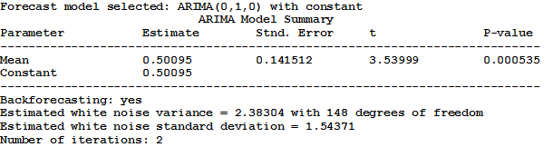
Clearly at least one order of differencing is needed to stationarize this series. After taking one nonseasonal difference--i.e., fitting an ARIMA(0,1,0) model with constant--the residuals look like this:

Notice that the series appears approximately stationary with no long-term trend: it exhibits a definite tendency to return to its mean, albeit a somewhat lazy one. The ACF plot confirms a slight amount of positive autocorrelation:

The standard deviation has been dramatically reduced from 17.5593 to 2.38 as shown in the Analysis Summary:

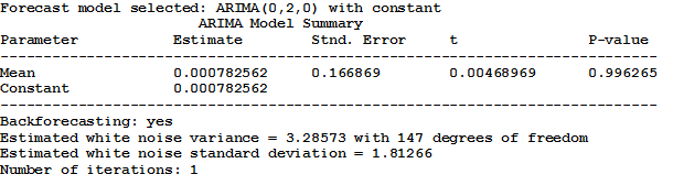
Is the series stationary at this point, or is another difference needed? Because the trend has been completely eliminated and the amount of autocorrelation which remains is small, it appears as though the series may be satisfactorily stationary. If we try a second nonseasonal difference--i.e., an ARIMA(0,2,0) model--just to see what the effect is, we obtain the following time series plot:

If you look closely, you will notice the signs of overdifferencing--i.e., a pattern of changes of sign from one observation to the next. This is confirmed by the ACF plot, which now has a negative spike at lag 1 that is close to 0.5 in magnitude:

Is the series now overdifferenced? Perhaps so, because the standard deviation has actually increased from 1.54371 to 1.81266:

Thus, it appears that we should start by taking a single nonseasonal difference. However, this is not the last word on the subject: we may find when we add AR or MA terms that a model with another order of differencing works a little better. (Adding an AR term corrects for mild under-differencing, while adding an MA term corrects for mild overdifferencing.) Or, we may conclude that the properties of the long-term forecasts are more intuitively reasonable with another order of differencing (more about this later). But for now, we will go with one order of nonseasonal differencing.

Go to next topic: Identifying the orders of AR or MA terms.