 ARIMA models for time series forecasting
Notes
on nonseasonal ARIMA models (pdf file)
Slides on seasonal and
nonseasonal ARIMA models (pdf file)
Introduction
to ARIMA: nonseasonal models
Identifying the order of differencing in an ARIMA model
Identifying the numbers of AR or MA terms in an ARIMA
model
Estimation of ARIMA models
Seasonal differencing in ARIMA models
Seasonal random walk: ARIMA(0,0,0)x(0,1,0)
Seasonal random
trend: ARIMA(0,1,0)x(0,1,0)
General seasonal models: ARIMA (0,1,1)x(0,1,1) etc.
Summary of rules for identifying ARIMA models
ARIMA models with regressors
The
mathematical structure of ARIMA models (pdf file)
Seasonal random trend
model: ARIMA(0,1,0)x(0,1,0)
Often a
time series which has a strong seasonal pattern is not satisfactorily
stationarized by a seasonal difference alone, and hence the seasonal random walk model (which predicts the seasonal
difference to be constant) will not give a good fit. For example, the seasonal difference of the deflated auto sales series
looks more like a random walk than a stationary noise pattern. However, if we
look at the first difference of the seasonal
difference of deflated auto sales, we see a pattern that looks more-or-less
like stationary noise with a mean value of zero:

(Even if
the mean value of a twice-differenced series is not exactly zero, we normally
assume it is zero for forecasting purposes: otherwise we would be assuming a
trend-in-the-trend, which would be dangerous to extrapolate very far.)
For
monthly data, whose seasonal period is 12, the first difference of the seasonal
difference at period t
is (Yt - Yt-12) – (Yt-1 - Yt-13). Applying the
zero-mean forecasting model to this series yields the forecasting equation:
(Ŷt - Yt-12 ) - (Yt-1 - Yt-13)
= 0
Rearranging
terms to put Ŷt by itself on the left, we obtain:
Ŷt =
Yt-12 + Yt-1 –
Yt-13
For
example, if it is now September '96 and we are using this equation to predict
the value of Y in October '96, we would compute:
ŶOct96 = YSep96 + (YOct95 – YSep95)
In other
words, October's forecast equals September's value plus the
September-to-October change observed last year. Equivalently, we can rewrite
this as:
ŶOct96 = YOct95 + (YSep96 – YSep95)
which says
that October's forecast equals last October's value plus the year-to-year
change we observed last month.
This
forecasting model will be called the seasonal random trend model,
because it assumes that the seasonal trend (difference) observed this month is
a random step away from the trend that was observed last month, where the steps
are assumed to have mean zero. To see this, rewrite the equation in terms of
seasonal differences:
(Ŷt - Yt-12 ) = (Yt-1 - Yt-13)
In other
words, the expected seasonal difference this month is the same as the seasonal
difference observed last month. Now compare this behavior with that of the seasonal random walk model: the seasonal random walk
model assumes that the expected values of all future seasonal differences are
equal to the average seasonal difference calculated over the whole
history of the time series. In contrast, the seasonal random trend model
assumes that the expected values of all future seasonal differences are equal
to the most recently observed seasonal difference. Moreover, the
seasonal random trend model assumes that the actual seasonal differences will
be undergoing a zero-growth random walk--rather than fluctuating around some
constant mean value--so their values will become very uncertain in the distant
future.
The
seasonal random walk model and the seasonal random trend model both predict
that next year's seasonal cycle will have exactly the same shape (i.e., the
same relative month-to-month changes) as this year's seasonal cycle. The
difference between them is in their trend projections: the seasonal
random walk model assumes that the future trend will equal the average
year-to-year trend observed in the past, whereas the seasonal random trend
model assumes that the future trend will equal the most recent
year-to-year trend.
Returning
to our example, if our last recorded value was for September '96, the seasonal
random trend model will predict October's value to satisfy (YOct96
– YOct95) = (YSep96
– YSep95). If we then
bootstrap the model one month into the future to predict November's value, the
model will predict that (YNov96 – YNov95) = (YOct96 – YOct95) ...but this is
exactly equal to (YSep96 –
YSep95)
again, because the October '96 forecast must be used in place of an actual
value. Thus, all future seasonal differences, as predicted from time
origin September '96, will be identical to the September-to-September
difference.
The seasonal
random trend model is a special case of an ARIMA model in which there is one
order of non-seasonal differencing, one order of seasonal differencing, and no
constant or other parameters--i.e., an "ARIMA(0,1,0)x(0,1,0) model."
In Statgraphics, you would specify a seasonal random trend model by choosing ARIMA
as the model type and then selecting:
- Differencing:
Nonseasonal Order = 1, Seasonal Order = 1
- AR,
MA, SAR, SMA = 0
- Constant
= off
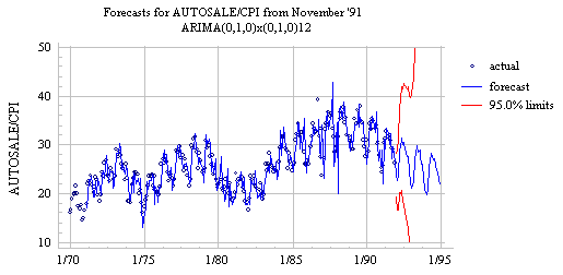
If we
apply the seasonal random trend model to the deflated auto sales data, using
data up to November '91, we obtain the following picture:

Notice
that the one-step-ahead predictions (up to November '91) respond very quickly
to cyclical upturns and downturns in the data, unlike those of the seasonal
random walk model. Also notice that the predictions for future seasonal cycles
have exactly the same shape as the last observed seasonal cycle (the one ending
in November '91). However, the long-term forecasts march off with a downward
trend equal to the downward trend that was observed from November '90 to
November '91. The confidence limits for the long-term forecasts also diverge
very rapidly because of the assumption that the actual future trend will be
randomly changing.
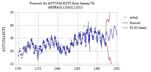
If we
recompute the forecasts using data up to January '92, we see a very different
picture in the long-term forecasts:

The upward
trend between January '91 and January '92 now causes the long-term forecasts to
shoot off upward! Thus, we see that the seasonal random trend model is much
more responsive than the seasonal random walk model to sudden shifts in the
data. This serves it well when forecasting one period ahead, but renders it
rather unstable for purposes of forecasting many periods ahead.
If you are
thinking at this point that it probably would be better to do some amount of smoothing
when estimating the seasonal pattern and/or the long-term trend in the
forecasts, you are right. (By "smoothing" I mean that you might want
to average over the last few season's data when estimating the seasonal pattern
and/or the trend.) You can smooth the trend estimate by adding MA=1 to
the parameter specifications, and you can smooth the estimate of the seasonal
pattern by setting SMA=1. Adding both of these terms will yield an
"ARIMA(0,1,1)x(0,1,1) model," which is probably the most commonly
used ARIMA model for seasonal data. (For the technically curious, setting MA=1
adds a multiple of the one-month-prior forecast error to the
right-hand-side of the forecasting equation, while setting SMA=1 adds a
multiple of the 12-month-prior error, and adding both terms together
also causes a multiple of the 13-month-prior error to be included. The
resulting model is a kind of "seasonal linear exponential
smoothing.") The forecasts generated by this model from time origin
November '91 indeed show a smoother seasonal pattern, a more conservative trend
estimate, and narrower confidence intervals:

The
preceding qualitative observations are confirmed by the model
comparison report for the seasonal random walk, seasonal random trend, and
more elaborate ARIMA models fitted to the deflated auto sales data. The
seasonal random trend model outperforms the seasonal random walk model within
the estimation and validation periods (i.e., for all one-step-ahead forecasts),
and the more elaborate models with additional ARIMA parameters improve on the
simpler models without those parameters. (Return to top of
page.)
Go to next topic: General
seasonal ARIMA models